1. INTRODUCTION
The current Colombian economy depends heavily on oil revenues (Rodríguez, D., 2022); in fact, the country's oil revenues from 2014 to 2021 corresponded on average to $ 2052 MMusd, equivalent to 0.9% of GDP (MinHacienda, 2022). Likewise, fuel exports and other industrial products accounted for 51% of the total value of exports (DANE, 2023). This means that the hydrocarbon production chain plays a major role for various sectors, both economically and sociall 2023). According to the DANE, fuel imports from January to June 2023 have reported values of US$ 34,719 MMusd, resulting in an 8% growth in gasoline, diesel, and jet consumption, compared to the same period in 2022 (DANE, 2023). This growing demand for fuels generates an opportunity for domestic refinery production, as well as for its contribution to the country's GDP.
The production of commercial fuels in Colombia is governed by different regulations, including document CONPES 3943 of 2018 (CONPES, 2018). This document establishes a gradual decrease of the content of sulfur compounds in commercial fuels; by 2025 and 2030, commercial diesel and gasoline fuels, respectively, must have a maximum content of 10 ppm. The reduction of sulfur content in fuels, at an industrial level, is carried out by means of hydrotreatment. Hydrotreating requires H2, which is produced from steam methane reforming (SMR). An increase in H2 production leads to an increase in the production of low sulfur fuels, leading to higher financial indicator values. An extra 2 MMSCFD of H2 production would allow an additional 2000 bls/month of ALC (light cycle oil) hydrotreating, a low commercial value intermediate product that is capitalized as a component in the diesel blending, increasing the production of high value products with a change in the gross refining margin of +$ 1.4 MMusd/month (2023 average TRM: $ 4020 cop/ usd). However, an increase in H2 production in an SMR industrial unit is conditioned not only by feedstock availability, but also by heat transfer effects on the furnace and the preheater train, especially in units that have been operating for a long time, which is referred to as EOR (end of run) (Janbarari & Najafabadi, 2023).
The operating efficiencies of industrial SMR units are limited in EOR operation, mainly due to catalyst and preheater train equipment fouling (Janbarari & Najafabadi, 2023). This fouling causes the flue gases to remove the heat available for the reforming reactions and for it to be discharged into the atmosphere at an elevated temperature, thus decreasing the efficiency of the process. Unfortunately, the maintenance of the preheating train and the change of the catalyst in the reactor require a total shutdown of the unit. The dependence on fuels makes the reforming operation critical for the economic and social sustainability of the country, restricting the unit shutdowns to the minimum possible. Therefore, the extended operation time, and the increase in H2 generation in EOR condition are required, while the respective supply plans are being executed. One possibility for the operation of SMR units in EOR conditions - maintaining methane, steam and fuel flows and considering heat transfer restrictions - is the identification of conditions that lead to an increase in H2 production. Such identification of conditions can be based on the analysis of operating data and on the results of a simulation for the furnace-train preheater system.
2 THEORICAL FRAMEWORK
STEAM METHANE REFORMING
SMR is the most common route in industry to obtain hydrogen (gray or blue); nearly 75% of the world's H2 production is carried out by this means (Fan et al., 2016). The most widely used CH4 source in the process corresponds to natural gas (Rostrup-Nielsen & Christiansen, 2011). The SMR process consists of causing a methane/steam mixture to react by using a catalyst, usually Ni on alumina (Soloviev et al., 2018), inside the tubes of a furnace called reformer. The reacting system, defined by equations (1-3) is endothermic (329.8 kJ/mol methane) and reversible, generating H2, CO and CO2 (Rostrup-Nielsen & Christiansen, 2011). The reformer output stream (syngas) is cooled and sent to a converter, where water and CO react giving way to more H2 and CO2 (equation 3, water-gas shift) (Shillawala et al., 2017; Amran et al., 2017). The H2-rich converter output stream is used for steam generation, through heat exchange, before being purified in an operation such as PSA (Moskowitz et al., 2015; Rostrup-Nielsen and Christiansen, 2011); the waste gases (CO, CO2 and CH2) from this operation are used as fuel in the reforming furnace.
At an operational level, CH4 conversion is favored by an excess of steam, a decrease in total pressure, and an increase in temperature; likewise, CO conversion (equation 3) is favored by an excess of steam and a decrease in temperature. Thus, the excess steam (steam to natural gas ratio) corresponds to a key variable for adjusting the H2 output obtained from the SMR process. The mass steam to natural gas ratio should range between 2 and 6 (Rostrup-Nielsen and Christiansen, 2011). If the ratio is below its minimum value, the charge will coke, poisoning the active sites of the catalyst. On the other hand, a steam/charge ratio above the upper limit increases the energy requirement and the pressure drop in the furnace tubes, resulting in a higher production cost and a lower economic benefit.
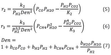
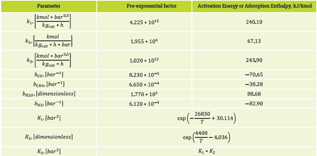
Regarding reaction kinetics, Xu & Froment (1989) developed a Langmuir-Hinshelwood type model, expressed in equations 4-7. This model considers the parallel occurrence of reactions (1-3) over a Ni/ Mg catalyst supported on alumina. The model (4-7) has been used in different SMR process simulations at industrial level (Posada & Manousiouthakis, 2005; Rostrup-Nielsen and Christiansen, 2011; Fan et al., 2016; Shillawala et al., 2017; Amran et al., 2017; Faheem et al., 2021).
Table 1 Constants for the kinetic model proposed by Xu & Froment (1989).
Source: Posada & Manousiouthakis, 2005.
In the kinetic model, P¡ corresponds to the partial pressure of component i. b f corresponds to the adsorption constant for component i. k 1t k 2 , k 3 correspond to the kinetic constants for reactions (1-3), respectively. K 1 , K 2 , K 3 correspond to the equilibrium constants for reactions (1-3). The values for the kinetic constants and equilibrium constants of the kinetic model (4-7) are shown in Table 1.
IDENTIFICATION OF OPERATIONAL MODES
The kmeans algorithm is a cluster identification method that can be used for different purposes such as definition of operational states in industrial processes (Lund & Ma, 2021; Jesper et al., 2021), identification of process failure (Gokilavani & Bharathi, 2021), identification of stationary states (Li et al, 2020), and outlier sample detection (Iftikhar et al., 2020). kmeans divides the data into k clusters such that the sum of distance between the data in the clusters is maximal, while the internal distances (from the data to their center in a cluster) are minimal (Thakare & Bagal, 2015). One of the most commonly used distances is the Euclidean distance. The k clusters are obtained in an iterative algorithm with a point of k centroids as the initial starting point. Defining the number of proper clustering can be done with the silhouette coefficient, S, (silhouette coefficient), which determines whether the samples are properly clustered (Dalmaijer et al., 2022; Rao & Govardhan, 2015); a sample is clustered successfully when S, is close to unity. The proper number of clusters is selected according to the maximum value of S averages over total data (Rao & Govardhan, 2015). On the other hand, a S value close to 0 indicates the sample belongs to several clusters; a negative S value indicates an erroneous clustering for the respective sample (Dalmaijer et al., 2022).
3 STATE OF THE TECHNIQUE
Hydrogen generation has gained importance in recent years for being an option as an energy source with low environmental impact (Fan et al., 2016). Analyses in H2 production by SMR process using simulation tools have been aimed at:
Energy integration: Posada & Manousiouthakis, 2005, proposed and modeled a heat exchange network with greater utilization of flue gases, reporting a potential decrease of ca. 36% in the cost of industrial services. Song et al., 2015, proposed improvements in the SMR process including the H2 purification PSA section from the simulation of an energy integration. The proposal focused on the compression of process gases that come from the reforming furnace before entering the preheating section, and the recovery of energy in the PSA equipment by means of a heat pump. According to Song et al. the proposed integration decreases by 40% the energy requirements (30% of the operating costs) of a conventional industrial process.
Decreased environmental impact: Fan et al., 2016, applied an exergy analysis to an SMR process considering combustion with oxygen carriers (CLC, chemical looping combustion) in the furnace.
With the CLC scheme, these authors obtained a CO2 separation with minimum extra energy requirement, decreasing the generation of greenhouse gases. Likewise, Chilliwala et al., 2017, analyzed the integration of SMR with dry methane reforming by simulation. According to the results of simulations, integration between these processes could lead to elimination in the formation of carbon deposits on the catalyst and high conversion of CO2 into valuable products with moderate energy consumption.
Feedstock change: Er-rbib et al., 2012, analyzed dry methane reforming in the production of synthetic fuels using computer simulation. According to the results, dry methane reforming has lower emissions than SMR, but higher energy consumption than SMR; also, according to the proposed operational scheme, dry reforming can lead to the generation of 72% synthetic diesel. It is important to note that the simulation was not validated. For their part, Ehteshami & Chan, 2014, presented a technical-economic analysis of the methanol, ethanol, and diesel reforming process, based on computational simulation results with the HYSYS program. According to the results, low temperatures for methanol reforming led to greater energy efficiency and economic benefit.
Advanced mathematical models for the reforming furnace: Kumar et al., 2016, developed an empirical model for online energy optimization of the SMR process. The model predicts the temperature distribution in the furnace based on fuel flow and calibration by infrared camera temperature readings. Likewise, the model was validated with measured data from an operating sample without presenting a statistical analysis. Kumar et al. stated that the application of the empirical model called EC-MR led to a 44% reduction in the non-uniformity of temperature distribution in a commercial furnace. These same authors (Kumar et al., 2017) applied a detailed model, with which they analyzed the spatial distribution of temperature in the reforming furnace. The model was validated without presenting a statistical analysis. The model was integrated into an optimization program of a standard reforming plant. Kumar et al. concluded that their model led to the reforming furnace being balanced in temperature distribution, with the respective increase in process efficiency.
According to the literature review, reports that use the simulation tool have focused on the analysis of more energy-efficient strategies, which can lead to a decrease in cost and increased economic benefits. A weakness identified in this review is the lack of explicit validation of the SMR process simulations with process data by means of variance analysis (ANOVA) and/or an F-test. Also, simulations have been performed on defined conditions for the industrial process, without mentioning possible different operating schemes underlying the process data.
4 COMPUTATIONAL DEVELOPMENT
DATA ANALYSIS
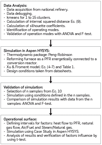
Process data for a reforming furnace and its preheater train at an SMR industrial unit of a national refinery were collected for an eight-year operating window. Samples with outliers were eliminated by interquartile range (Ewens & Brumberg, 2023). Also, the database was analyzed with the kmeans clustering method and the silhouette coefficient for the identification of operating modes representative of the unit. The different performances in H2 generation obtained with the identified operating modes were validated by means of ANOVA and F-tests, taking as H0: the equality between means and the ratio between variances equal to unity, respectively (Ewens & Brumberg, 2023; Box et al., 2008). The statistical procedures were applied according to the codes of the open-source R program (R Core Team, 2021) and its Rcommander package (Fox, 2017).
SIMULATION OF THE REFORMING FURNACE AND PREHEATING TRAIN
The reforming furnace and the preheating train of the SMR unit were simulated in the Aspen HYSYS v.10 program. The geometrical aspects of the equipment were taken from the respective specification sheets. Likewise, the operational conditions for the simulation were established according to the design condition. The thermodynamic package named Peng-Robinson was chosen due to different literature supports (Vlädan et al., 2011; Ehteshami & Chan, 2014; Challiwala et al., 2017). The reforming kinetics was established according to the Xu & Froment model for chemical equations (1-3), predominant in the furnace conditions (Barelli et al., 2008; Rostrup-Nielsen & Christiansen, 2011). The steam/natural gas ratio was set to 3.33, while the air/fuel ratio corresponded to 3.7. The natural gas and steam streams were mixed generating a 54000 lb/h stream at 510 °F and 425 psia to feed the reforming reactor, defined as a PFR reactor. The PFR was detailed with a length and total volume of 40 ft and 400 ft3, respectively. The PFR object was thermally connected to a conversion reactor. This reactor develops the burning of a 34000 lb/hr fuel flow at 1900 °F and 20 psia, supplying ca. 80 MMBTU/hr to the PFR reactor. Hence, the PFR and conversion reactor objects are thermally coupled, representing the operation of the reforming furnace. This coupling has been used in various Literature works (Posada & Manousiouthakis, 2005; Fan et al„ 2016; Challiwala et at, 2017; Amran et al„ 2017).
VALIDATION OF THE SIMULATION
The simulation developed was validated using samples of the process data for each operational mode (Section 4.1). The selection of the data was carried out according to the following formula for the calculation of the size of a finite sample (Taborga et al., 2011)
Where, n, m, p, q, N and e correspond to: reduced sample size, parameter according to the confidence level (for 0.05, m=1.96) probability in favor (0.5), probability against (0.5), initial sample size and estimation error (0.05), respectively. With the n samples, the respective simulations were performed to obtain the generated H2 flow. The simulations of the n samples were executed with the communication protocol between Excel and Aspen HYSYS, established in the Aspen Simulation Workbook add-in. The F-test was applied to compare the variances between the results of the simulations and the respective process data. The H0 corresponded to a ratio of variances between the sets equals to unity (Box et al. 2008). Complementarily, the one-way ANOVA test was applied to compare the means between the two data sets. The H0 in this case corresponded to equality between means (Box et al., 2008; Ewens & Brumberg, 2023).
GENERATION OF OPERATIONAL SURFACE
The operational surface of the reforming furnace and the preheating train of the SMR unit was obtained considering the following factors: combustion air flow, heat flow from the conversion reactor to the PFR reactor, natural gas flow, total air to fuel gas ratio, and steam to natural gas ratio. With the foregoing, the steam to natural gas and air to fuel gas ratios were changed from their initially established values (Section 4.2). The response variables for the operational surface corresponded to the H2, CH4, water, CO, and C02 flows at the PFR outlet, the PFR outlet temperature, and the flue gas temperature. The operational surface was obtained by the Case Study tool available in Aspen HYSYS. The different effects resulting from the variation of the factors were validated through the statistical t-test. The influence of the factors on H2 generation was analyzed from the operational surface obtained by simulation.
RESULTS
TRENDS IN PROCESS DATA
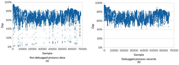
Table 2 presents the variables from process data, while Figure 2 llustrates the trend in H2 generation before and after the elimination of outliers. After debugging, the SC (steam/natural gas) ratio reported variation between 2.53 and 5.72, with mean value at 3.6 while the Air_Com (air/fuel gas) ratio presented values between 3.35 and 13.95, with mean at 4.57. These two variables, SC and Air_Com reported a high concentration of points (between the first and third quartiles) in the intervals 3.59-3.68 and 4.23-4.84, respectively. Values outside these zones can be considered unit operations in dynamic state or with measurement errors of the respective sensors. The high values presented, particularly, by the Air_Com variable may be related to a saturation of the flue gas system (100% opening of the flue gas system).
Table 2 Reforming furnace and preheating train operating variables.
| Variable | Description |
|---|---|
| ABA | Valve opening 1 flue gas outlet, %. |
| ABB | Valve opening 2 flue gas outlet, %. |
| Air_Com | Air/fuel mass ratio. |
| Cap | H2 generation reported by the operation (fraction or %). |
| CH4 | CH4 mass flow generation (Lbmol/h). |
| CO | CO mass flow generation (Lbmol/h). |
| C02 | C02 mass flow generation (lbmol/h) |
| H2 | H2 mass flow generation (lbmol/h). |
| Heat | Heat flow to PFR (MMBTU/h unless otherwise specified). |
| Mair | Combustion air mass flow (Lb/h). |
| Qgas | Reforming influent natural gas mass flow (lb/h). |
| QH2 | Volume flow of hydrogen in the reforming effluent syngas (MMSCFD). |
| QPSA | Reforming effluent synthesis gas volume flow rate (MMSCFD or lbmol/h). |
| SO | Steam/natural gas mass flow ratio. |
| TFG | Flue gas temperature (°F). |
| TePFR | PFR reaction gas inlet temperature (°F). |
| TsPFR | PFR reaction gas outlet temperature (°F). |
Source: Authors.
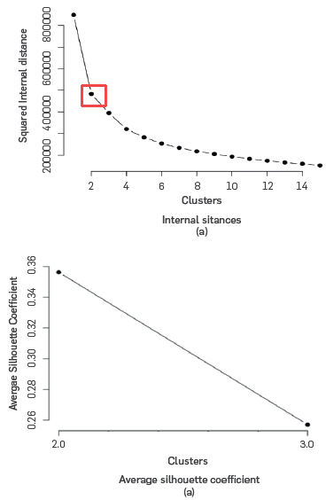
Figure 3a shows the variation of the internal distance of the clusters versus the number of clusters, according to the results of the kmeans method. According to this figure and the elbow method a number of two clusters or modes represent the operation of the SMR industrial unit. The information obtained with the third cluster is negligible compared to that obtained with two clusters. Complementarily, Figure 3b presents the average silhouette coefficient for two and three clusters. Accordingly, the average silhouette coefficient for two clusters is larger than the coefficient for three clusters, which confirms that the SMR unit data can be organized into two operating modes.
Source: Authors.
Figure 3 Variation of the sum of internal distances squared vs clustering by kmeans.
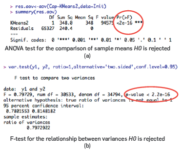
On the other hand, Figures 4a-b show the results reported by the R program for the validation of the differences in performance between the two operating schemes, by means of ANOVA and F-tests. According to the results, the H0 of equality of H2 production means (Cap) is rejected due to the value of the p-statistic (p<0.05) (Figure 4a). Likewise, the H0 of ratio between population variances of H2 productions equals to unity is rejected according to the respective p-value (p<0.05) (Figure 4b). Therefore, the two schemes lead to different population means and their distributions have different variances; i.e., the two operational modes obtained with the kmeans method generate statistically different performances.
FURNACE AND PREHEATING TRAIN SIMULATION.
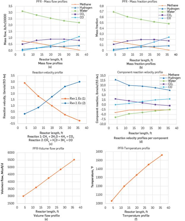
Figure 5 presents the simulation PFD developed in Aspen HYSYS for the furnace and the preheater train, reporting convergence for the design operating conditions of the SMR industrial unit. Figures 6a-b illustrate the longitudinal profiles of mass flows and compositions for the PFR (reforming furnace). Figures 6c-d present the profiles of reaction rates and component rates in the reforming furnace, while Figures 6e-f show the trends for the volumetric flow and temperature along the PFR reactor.
VALIDATION OF THE SIMULATION
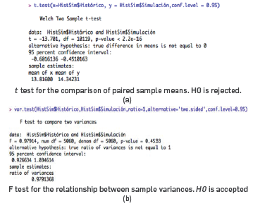
A number of 5097 random samples from the process data were used in the simulation for the respective calculation of the H2 flow output of the PFR; the samples were selected without distinction between operating modes 1 and 2. From the samples taken, 36 reported null convergence in the simulation, which represents 0.7% of the total. Figure 7a presents the H2 flow dispersion of the data and the simulation results for the 5061 samples that resulted in convergence, while Figure 7b compares the values of these flows in the boxplot. According to these figures, the simulation prediction shows a close match to the process data. The t and F statistical tests compare the means and variances of the 5061 operational samples with the simulation results; the H0 corresponded to the difference between means equal to zero and the ratio between population variances equal to unity, respectively. The results of the statistical tests are shown in Figures 8a-b. According to these figures, the H0 of equality of population means is rejected (p<0.05), but the H0 of unit ratio of population variances is accepted (p>0.05).
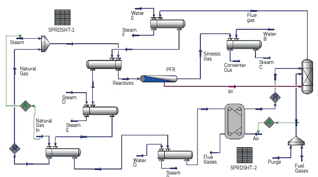
Figure 5 Process flow diagram defined in Aspen HYSYS for the furnace and preheating train of the SMR industrial unit.
Source: Authors.
Figure 6 Profiles resulting from the simulation with the SMR unit furnace design conditions.
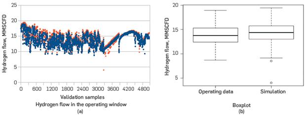
Figure 7 Comparison of hydrogen flow values from historical (blue) and simulation results (red) for the 5061 randomly selected samples. Red: simulation; Blue: historical.
OPERATIONAL SURFACE
The operational surface was determined based on the ranges for operational mode 1, which has the highest average H2 production values. Table 3 defines the levels for each factor used in the Case Study analysis at Aspen HYSYS; these levels coincide with the typical ranges for industrial units (see Rostrup-Nielsen and Christiansen, 2011). Each of these factors were analyzed at three levels, which generated 35=243 case studies for the simulation.
Table 3 Factors and levels to obtain the operating surface with simulation.
| Factor | Design Value | Lower level (-) | Medium level (0) | Higher level (+) |
|---|---|---|---|---|
| Air flow (Mair), lb/h | 115800 | 46000 | 92500 | 139000 |
| Air/fuel (Air_Com) | 3.33 | 3.0 | 3.5 | 4.0 |
| Natural gas flow to reformer (Qgas), lb/h | 12390 | 11265 | 12517 | 13768 |
| Steam/natural gas (SC) | 3.7 | 2.5 | 3.75 | 5.0 |
| Heat flow to PFR (Heat), MMBtu/h | -78.56 | -62.85 | -78.56 | -94.27 |
Source: Authors.
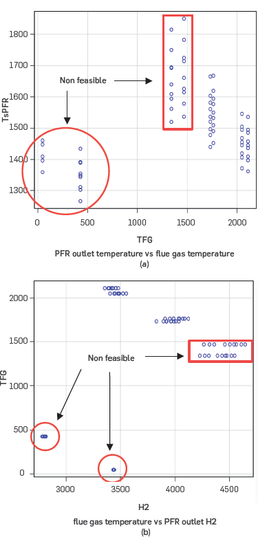
The results of the Case Study run show convergence of the simulation for most of the combinations between factors and levels. Out of 243 cases, the simulation did not achieve convergence in 39 cases, as the air flow did not report compliance with the required heat flow requirement for the PFR. Also, Figures 9a-b show the scatter plot between the PFR reactor outlet temperature and the conversion reactor flue gas temperature (TFG) and TFG vs PFR outlet H2, respectively.
OPERATIONAL MODES
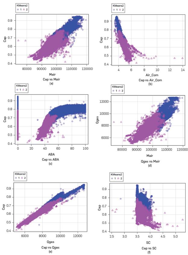
According to section 5.1, the representation of the process data by two operational modes is supported by the calculation of the silhouette coefficient and by statistical tests. Thus, although the data come from the same unit, the ranges of the variables lead to the operating modes having different population means, due to differeces in the conversions of the two reactions (equations 1 and 2). Although H2 is generated in the two reactions, appreciable quantitative differences are obtained due to the stoichiometry of the reactions. The trends of the hydrogen generation variable (Cap) with different operational variables, in the two operating modes defined with kmeans, are shown in Figures 10a-f. According to these figures, operating moNe 1 (42% of the samples) is characterized by higher hydrogen production values than operating mode 2 (58% of the samples). Similarly, mode 1, compared to mode 2, exhibits higher values for the variables Mair, Qgas and ABA (Figures 10a,c,e), but presents lower Air_Com ratio values (Figure 10b). The lower Air_Com values in operating mode 1 lead to higher energy transfers to the reforming reaction, with a corresponding elevation in hydrogen generation. Natural gas flows to reforming and combustion air flows above 9000 lb/h and 105000 lb/h, respectively, lead to H2 generation capacities above 80% (Figures 10a-e). Also, for these capacities, the stack gas control system reports openings above 60% (Figure 10c). Likewise, for a flow of natural gas to reformed gas, the operation reports the use of a combustion air value4ranging betwe4e5n 100±10 klb/h (Figure 10d). On the other hand, the SC variable does not exhibit characteristic intervals according to the clusters; however, from Figure 10f, it is possible to infer that thee highest hydrogen production is obtained with low SC values (steam/natural gas ratio), due to higher temperature in the reforrmer.
FURNACE AND PREHEATING TRAIN SIMULATION
According to Figure 6a, the mass flows of the reagents, methane and water, decrease, which generates an increase in the flows of H2, CO2, and CO with reactor length, in agreement with the works of Singh et al., 2014 and Abbas et al., 2017. The mass slope of water decrease is larger than the mass slope of CH4 decrease (Figure 6a), which was expected due to the stoichiometry of the reactions and the molecular weight of these reagents; this decrease is less marked in terms of mass fractions (Figure 6b) due to the excess of water vapor in the reaction mixture (approximately 70%). The consumption and generation profiles indicate the progress of the reforming reactions in the reforming furnace piping.
In accordance with different references (Challiwala et al., 2017; Amran et al., 2017; Abbas et al., 2017; Singh et al., 2014), reaction 1, CH4 + 2H2O = 4H2 + CO2, presents its highest velocity at the furnace entrance and decreases with the advance in pipe length (Figure 6c). The velocity of reaction 1 changes sign after 32 ft of pipe length, whereby the reversible direction begins to dominate, decreasing the amount of H2 generated by this reaction. Despite this consumption, H2 production continues to increase due to the advance of reaction 2 (Abbas et al., 2017; Singh et al., 2014). Similarly, the change in the CO2 trend from production to consumption is observed from 32 ft (Figure 6d); this decrease in selectivity towards CO2 coincides with literature reports (Minette et al., 2018; Kumar et al., 2017; Lao et al., 2016; Abbas et al., 2017; Wang et al., 2021). Meanwhile, reaction 2, CH4 + H2O = 3H2 + CO, presents its lowest velocity at the furnace entrance, increasing its profile with length progress (Figure 5c). The trends of reactions 1 and 2 with length coincide with the increase in temperature, along the length of the tubes, as shown in Figure 6f and as presented by the literature (Minette et al., 2018; Singh et al., 2014). Considering the combined effect of reaction 1 and reaction 2, the H2 generation rate decreases with the advance in pipe length (Figure 6d), as a consequence of the decrease in the rate of reaction 1, which contributes an additional 0.33 moles H2 / mol CH4 consumed, compared to reaction 2. The decreasing trend in H2 generation rate does not affect the methane consumption rate profile, which remains nearly constant from 10 ft of pipe length (Figure 6d); each reaction has a unit stoichiometric coefficient for methane. Unlike CH4 consumption, water consumption is decreasing (Figure 6d) due to the increase in the rate of reaction 2, which, compared to reaction 1, requires 1 mol less water.
Likewise, the advance of the reforming reactions causes an increase in the volumetric flow and temperature profiles (Figures 6e-f), The increase in volumetric flow results from a combination of the increase in molar flow, due to the effect of stoichiometry, and the increase in temperature due to the energy supply from combustion (371 kJ/mol of methane consumed according to simulation results, coinciding with that reported by Posada & Manousiouthakis (2005). This increase in temperature is almost linear characteristic of a near equilibrium state (Figure 6f), coinciding with that reported by Wismann et al. (2019) and Faheem et al. (2021). This profile results as a consequence of a uniform energy distribution along the PFR reactor, assumed by Aspen HYSYS. At the industrial level, the heat distribution in the reformer tubes is not homogeneous, with the heat flow decreasing with tube length (Rostrup-Nielsen and Christiansen, 2011; Lao et al., 2016; Wang et al., 2021). This causes an increasing temperature profile that tends to stabilize at the end of the reformer tube length (see Lao et al., 2016; Wang et al., 2021), differing from that obtained by simulation with Aspen HYSYS (Figure 12b). Despite this disparity in temperature profiles, the prediction of the variation in compositions and reaction rates agrees with the published works (Rostrup-Nielsen and Christiansen, 2011; Lao et al., 2016; Wang et al., 2021). The comparison between the information for the design condition of the SMR unit and the results obtained by the simulation with Aspen HYSYS are shown in Table 4. According to this Table, the amount of H2 generated and the amount of CH4 consumed are reproduced with errors of 5,5% and 9,6%, respectively; however, on average, the errors in the flow predictions correspond to 3.5%, which is in the tolerance range for process simulators (Amran et al., 2017; Abbas et al., 2017; Zhu et al., 2015; Singh et al., 2014).
Table 4 Comparison of design data with simulation results in Aspen HYSYS.
Source: Authors.
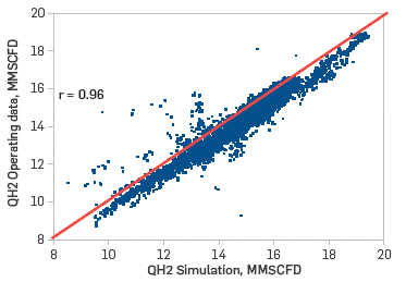
As shown in section 5.3, the comparison between simulation predictions and process data reported the rejection of H0 for equality of population means (Figure 8). The non-equality between population means may be a consequence of the inclusion of samples from the two operational modes, as well as possible samples in dynamic state in the validation sample set. Hence, the t test was repeated separately with the samples corresponding to each mode, reporting p-values>0.05 for the two operational modes. In this regard, the differences between the model assumptions (constant feed properties, homogeneous heat distribution and one-dimensional variation in the PFR, as well as no heat loss to the environment) and the industrial day-to-day operational situations (change of compositions in the feed streams, sensor errors, piping and insulation damage, disturbances, EOR condition) must be considered. Due to such differences, the statistical t test reports mismatch between the means of the data obtained by simulation and the process data. Nonetheless, from Figure 7a, it is possible to state that the trend reported by simulation for H2 generation reproduces the trend contained in process data. In fact, the parity graph shown in Figure 11 details a concentration of prediction points near the 45° line, which brings the simulation close to process values. Likewise, the parity graph shows a tendency in the simulation to overestimate the hydrogen flows, with respect to those contained in the process data. This overestimation can also be inferred from the boxplot (Figure 7b). This overestimation is related to the EOR condition of the industrial unit.
In quantitative terms, the average simulation prediction errors correspond to 8.2%; different authors assume that the simulations reproduce the operational data at a semi-quantitative level, with average error values below 10% (Amran et al., 2017; Abbas et al., 2017; Zhu et al., 2015; Singh et al., 2014). From the above and, considering the match between the concentration and velocity profiles (Figures 6a-b), it can be stated that the simulation reproduces the H2 generation data of the SMR industrial unit at a semi-quantitative level. It is worth mentioning that the comparison of simulation results with operation data for an SMR industrial unit, developed in this work, is the first one reported in the literature, according to the review conducted with different publishers; usually, simulations are compared with point samples.
ANALYSIS OF THE OPERATING SURFACE
Figure 9 shows the simulation cases with convergence that report unfeasible results due to the temperature crossover in the reforming furnace (higher temperature in the PFR than in the converter). These temperature crossovers occur at the upper level of the heat flow. Nevertheless, the simulator reports convergence since the coupling between the PFR and converter reactors, which simulates the reforming furnace, was performed using an energy stream (see counterpart simulations in Posada & Manousiouthakis, 2005; Fan et al., 2016; Challiwala et al., 2017; Amran et al., 2017; Faheem et al., 2021). The energy stream does not consider the constraint between flue gas temperatures and PFR output. This deficiency in the simulation with Aspen HYSYS and other commercial packages had not been explicitly highlighted in previous research.
As stated above, simulations with commercial packages are validated with point samples and then used to explore changes in concentration or other variables that do not involve changing the thermal coupling conditions between the PFR and the conversion reactor. On the other hand, the constraint on temperature crossover can be considered in an optimization scheme with the same computational packages (Posada & Manousiouthakis, 2005). Kumar et al., 2016, and Kumar et al., 2017, applied CFD simulations of the furnace, including the reforming reactions in the tubes, which favors the analysis of the constraints on flue gas and syngas temperatures. It also reproduces a temperature profile in the furnace tubes in line with that reported for industrial units (Lao et al., 2016; Wang et al., 2021). Therefore, this kind of simulation application or coupling is recommended for future work related to H2 generation in reforming furnaces.
Source: Authors.
Figure 11 Parity graph for volumetric hydrogen flow, operating data versus simulation.
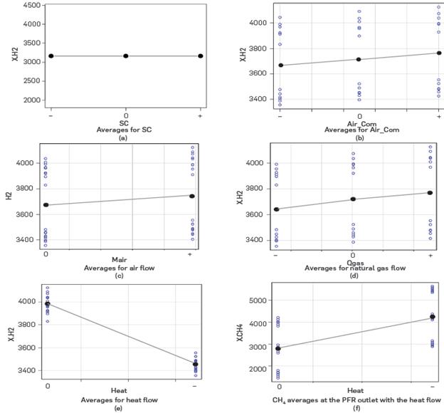
Consequently, the cases with temperature crossover between the flue gas and the synthesis gas were excluded from the operational surface, reducing the number of feasible cases for analysis to 107. The effects of the factors were analyzed from the feasible cases. The averages of the effects of the individual factors on H2 generation are presented in Figures 12a-f. The analysis of these effects suggests that the SC (steam/natural gas) ratio has no influence on H2 generation at the levels assumed for the simulation (Figure 12a), agreeing with that reported by Zhu et al. (2015) and Abbas et al. (2017). According to Abbas et al., 2017, the SC factor does not present influence due to a possible compensation between the kinetics of reactions (1) and (2), maintaining the H2 production Levels, In industrial operations, the SC ratio is usually kept between 3 and 4 to minimize coke formation during reforming (Fan et al., 2016; Zhu et al., 2015). H2 generation decreases significantly for Lower values of the SC ratio (Rostrup-Nielsen and Christiansen, 2011).
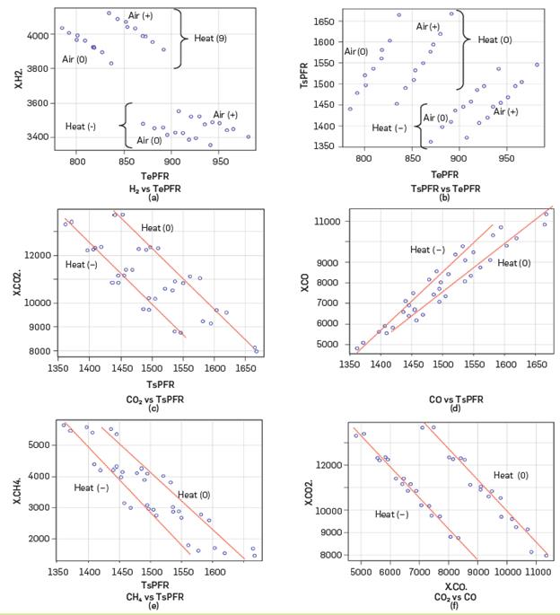
Figure 13 Relationship between the response variables according to the feasible results of Case Study.
On the other hand, the effects of Air_Com ratio, air flow, and natural gas flow on H2 generation are presented in Figures 12b-12d, respectively. These figures suggest a slight increase in H2 generation with the value of their respective levels. Although these factors affect the convection section of the furnace, a statistical t-test Leads to conclude that the influence of these factors on H2 generation is null at the analyzed Levels. Regarding the heat flow, Figures 12e-f show the influence of this factor on H2 generation as well as the CH4 outflow from the reactor. According to these figures, H2 generation ncreases with heat flow (from "-" to "0" level) in a statistically significant way, coinciding with what reported by Jabbour et al. (2017) and Faheem et al. (2021). On the other hand, although heat flow does not show a statistically significant influence on CH4 outflow, the trend shown in Figure 12f is in agreement with that reported by Jabbour et al. (2017), Faheem et al. (2021) and Rostrup-NieLsen and Christiansen (2011).
The trends between the response variables and various factors combined are shown in Figures 13a-f. Accordingly, the response variables present two separate trends, defined by the Lower ("-") and middLe ("0") Levels of heat flow to the PFR (Table 3). For the influence of the PFR inlet temperature factor, TePFR, on H2 generation (Figure 13a) and on the PFR outlet temperature, TsPFR, (Figure 13b) each heat flow Level presents two divisions, according to the middle ("0") and upper ("+") Level of air flow to the conversion reactor (i.e. the combustion process in the reformer). It follows from Figure 13a that H2 generation increases with decreasing TePFR and increasing heat flow to reactor; Likewise, an increase in air flow allows keeping H2 generation constant with increasing TePFR. Conversely, according to Figure 13b, the TsPFR increases with increasing TePFR and heat flow. Likewise, TsPFR can be kept at certain level by increasing air flow and increasing TePFR. The influence of air flow on the response variables shows the dependence of the reforming reaction on the combustion process in the furnace. This had not been explicitly considered in previous simulations of the SMR process.
SimiLarly, according to Figures 13c-e, an increase in TsPFR Leads to a decrease in CO2 outflow, an increase in CO outflow, and a decrease in CH4 outflow, respectively, matching the experimental profiles reported by Jabbour et all. (2017). SimiLarly, an analysis of these figures suggests that an increase in heat flow Leads to maintaining the values of CO2, CO, and CH4 outflows for higher values of TsPFR. Figure 13f suggests that CO2 flow decreases with CO flow but increases with heat flow. The trend between these CO2 and CO flows in Figure 13f is consistent with the competition between the reforming reactions. SimiLarly, the H2/CO ratio takes values below unity (between 0.3 and 0.9), which is subsequently adjusted, to values between 3 and 5, by means of a reactor favoring the water-gas-shift reaction (equation 3) (Rostrup-Nielsen and Christiansen, 2011), not included in this work.
In sum, the analysis of the operational surface with the feasible cases suggests that H2 generation is influenced by the heat flow coming from the conversion reactor. Also, the feasible cases suggest a competition between the reforming reactions (1 and 2). In operation, a rise in flue gas temperature with excess air Leads to a decrease in heat flow to the PFR, with an increase in H2 generation by favoring reaction 1. The favoring of reaction 1 means an increase in the synthesis gas outlet temperature (TsPFR) due to the Lower energy requirement (165 kJ/mol). When reaction 2 is favored, the TsPFR decreases due to the higher energy requirement (206 kJ/mol).
Abbas et al., 2017, in their pilot level experiments and Zhu et al., 2015, in their analysis of an industriall plant by simulation, report a stationary zone in H2 generation for moderate temperatures and heat flows. To deepen this aspect, the analysis of the operational surface was complemented with indoor Levels in the intervals defined for the factors (Table 3). The feasible cases with convergence in the new Case Study (66 feasible cases) were grouped with those of the previous one (108 feasible cases). Figure 14 presents the trends obtained with all the feasible cases (174) for H2 generation with respect to heat flow and natural gas flow to reforming (parametrically). In this figure, the vertical points correspond to different values of natural gas to be reformed; the higher the Location of the point, the higher the value of natural gas to be reformed. According to Figure 14, the higher H2 generation is achieved with higher values of heat received and higher value of natural gas to reformed. However, the increase in H2 generation is stabilized with the higher values of heat and natural gas, tending to a steady state value (closer proximity between the vertical points). This result agrees with Abbas et al., 2017, and Zhu et al., 2015, reporting, validating the trends obtained by simulation for the operational surface. With the above, the simulation developed in Aspen HYSYS Leads to the prediction of an increase of up to 10% of the average H2 generation capacity, in EOR condition of the industrial unit.
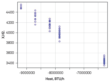
Figure 14 Variation of the H2 flow generated with the heat received in the PFR and the flow of reforming natural gas (circles for the same heat flow).
Finally, increasing H2 production also means increasing greenhouse gas emissions. The International Energy Agency has reported an emission factor for blue hydrogen production of 2 kg CO2-eq/kg H2 (IEA, 2019). Based on both this factor and the simulation results, an 10% increase in H2 capacity under EOR conditions will increase emissions from the unit process by 653 kg CO2-eq/h. For its part, the Mining and Planning Energy Unit (UPME) reported an emission factor of 112 kg CO2-eq/MWh from the electricity power grid in Colombia for 2022 (UPME, 2023). Considering the average electricity consumption for electrolysis of 52,2 kWh/1 kg H2 (IEA, 2019), hydrogen production from the grid would emit 5,84 kg CO2-eq/kg H2. Thus, the CO2 balance between increasing capacity and using H2 to generate electricity (not consuming electricity from the national grid) reports a value of -3,84 kg CO2-eq/kg H2. Taking into account the role of blue hydrogen in the country's energy transition, the capacity increase of the SMR unit in the EOR condition would contribute to a reduction of 1452 kg CO2/h or 12636 t CO2/year, contributing to the national decarbonization targets by 2030 (NDC, 2030).
CONCLUSIONS
Statistical analysis of process data collected from the furnace operation of an industrial steam methane reforming unit Led to the definition of usual operating ranges for steam/natural gas and air/ fuel gas ratios of 3.59-3.68 and 4.23-4.84, respectively. The air/ fuel gas variable also showed a direct relationship with the steam/ natural gas to reformed. Thus, as the mass ratio of air to total fuel increases, temperatures and the amount of hydrogen produced in the unit decrease. The application of the kmeans method Led to the proposal of 2 operating modes representative of SMR unit operation. The verification of the number of modes was performed using the average of the silhouette coefficients. Mode 1 (48% of the samples) was characterized by higher values of hydrogen generation and flue gas temperature than Mode 2 (52% of the samples). Mode 1 showed high values for the variables air flow and natural gas flow, while the air to fuel gas ratio showed Low values. The two modes occurred interchangeably throughout the period analyzed, showing a decreasing trend in hydrogen production over time. This decrease in hydrogen production is related to the fouling of the heat exchange equipment. Regarding the steam/natural gas to reforming, the trend of this parameter over the operating period did not distinguish between the different operating modes. The ANOVA and F statistical tests Led to the validation of the two operating modes obtained with the kmeans method.
The simulation developed for the furnace and the preheating train of the SMR industrial unit showed that reaction 1, CH4 + 2H2O = 4H2 + CO2, presents its highest velocity at the furnace entrance and decreases with the advance in the Length of the pipe, while reaction 2, CH4 + H2O = 3H2 + CO, presents its Lowest velocity at the furnace entrance, increasing its profile with the advance in the Length. The velocity of reaction 1 changes sign from 32 ft of pipe Length, whereby the reversible direction begins to dominate by consuming H2. Nonetheless, H2 generation continues to increase due to the advancement of reaction 2. The trends in methane consumption and hydrogen production decrease with reactor Length. Notwithstanding, the methane consumption rate remains constant from 10 ft reactor Length onwards. Statistical validation of the simulation was performed using randomly selected samples from the operational data. The H0 for the difference of the population means was rejected (p<0.05), which is a consequence between the model assumptions and the industrial day-to-day operation. However, the averaged errors of the flow predictions with the simulation corresponded to 8.2%, which is within the ranges reported in the Literature.
The exploration of the operating surface Led to the invalidation of some of the simulation results due to temperature crossovers between the PFR temperature and the conversion reactor temperature, which by their energetic coupling simulate the operation of the industrial reforming furnace. This deficiency in the simulation had not been explicitly highlighted in previous investigations. The analysis of the effects in the simulations with feasible cases showed that the higher H2 production was achieved with higher values of heat received in the PFR and higher value of natural gas to be reformed. However, the increase in H2 production was stabilized at the higher values of heat and natural gas, tending towards a steady state value. Increasing the PFR outlet temperature resulted in both a decrease in the CO2 production and an increase in the CO production. The distribution between the CO2 and CO production was consistent with the competition between the reforming reactions.


