


 English (pdf)
 Article in xml format
 Article references
 Send this article by e-mail
 Cited by SciELO
  Cited by Google
  Similars in
SciELO
Similars in
SciELO  Similars in Google
 Permalink
1. Introduction
Electric distribution networks provide electrical service to all end users in medium- and low-voltage levels [1,2]. Due to investment constraints in terms of utilities, these networks are built with radial topologies [3,4], and they include feeders with three-phase and single-phase configurations; however, these characteristics of the distribution networks increase their power losses when compared with transmission and sub-transmission power systems [5]. Usually, the strategies in distribution system operation are implemented to reduce grid power losses, but many of the research focus on the losses caused by current flow through lines (Joule effect) and neglect the important contribution of electric transformers [6-9]. Usually, parameters of electric transformers are unknown, and they are not considered in calculations for losses studies. Consequently, distribution transformers produce high values of power losses because utilities do not consider these devices for maintaining purposes; companies consider the importance of this device for quality purposes [10,11]. The electrical parameters in transformers can suffer critical changes caused by the deterioration in the coil insulation and dielectric paper [12-14]; they are provoked mainly by their lifetime (20-30 years), working all the time. and their permanent exposition to weather conditions depending on their place of installation [15,16]. It is clear that accurate models of the electrical networks are important to determine an adequate operation dispatch in the grids; these models include load measures and grid parameters (i.e., line and transformer models) [17]. For this reason, this research proposes an estimation strategy for determining the electrical parameters of single-phase transformers along the distribution grids using voltage and current measures. The main advantage here is that the transformers work continuously, implying that the quality index based on frequency and duration are not affected [15]. The advantage of the proposed approach to determine electrical parameters under steady-state operating conditions is that the measures of voltages and currents avoid the usage of open-circuit and short-circuits tests that are only possible in specialized laboratories the transformer.
In the specialized literature, the problem of parametric estimation in single-phase transformers has been formulated as a nonlinear programming model based on the application of Kirchhoff’s laws to the equivalent circuit of the transformer [18]. Here, we present some references regarding the parametric estimation in single-phase transformers.
The authors of [19] have proposed an optimization algorithm based on the bacterial foraging method to determine the internal parameters of the transformer. The numerical validation is made in a unique test feeder and the results are compared with the classical tests of short- and open-circuit. Authors of [20] have proposed a real-time estimation strategy for the parametric estimation in transformers using voltage and current measures. For doing so, these authors have presented an interface implemented using the LABVIEW software. With this interface, they solved the equivalent differential equations that model the distribution transformer using an algorithmic procedure. It is important to mention that the parameters of the transformer estimated using this approach have errors of 5-10 % when they are compared with the classical laboratory tests.
In reference, [21] presented a design procedure for distribution parameters for medium-voltage levels from a constructive point of view. The authors used the parametric information on similar transformers available commercially as inputs to propose a nonlinear programming model that is solved iteratively. Numerical results obtained with the solution of this nonlinear programming model are comparable with the geometric characteristics of real transformers; this allows the improving of existing designs and proves a useful strategy for transformer manufacturers.
Authors of [22] suggested a heuristic optimization algorithm based on chaotic search to determine the electrical parameters in single-phase transformers. The main contribution of this research corresponds to the usage of voltage and current measures, used in the objective function that is formulated as the minimization of the mean square error between the electrical measures and the calculated voltage and current variables. Experimental validations demonstrate high-quality results of the proposed optimization procedure.
Authors of [15] have proposed a nonlinear programming model to estimate the parameters in single-phase transformers considering voltage and current measures. The main contribution of this approach is the formulation of the optimization problem using real variables, allowing its implementation in the GAMS software. Numerical results demonstrate the effectiveness of the proposed nonlinear programing model with numerical implementations in three different tests feeders. Other common approaches to determine the electrical parameters in single-phase transformers include the gravitational search algorithm [18], particle swarm optimization [22], coyote optimization algorithm [23], manta-ray foraging optimization, chaotic manta-ray foraging optimization methods [12], etc. Note that the main advantage of these approaches is the easy implementation using free programming software with sequential programming strategies that allow finding quality results with a low computational effort [15].
Unlike previous works, this paper proposes the application of the sine-cosine optimization algorithm to estimate the parameters in single-phase transformers by considering voltage and current measures; this is the main contribution of the research, since this algorithm has not been previously applied to this problem. In addition, numerical results show better objective function values when compared with the GAMS solutions reported in [15].
The rest of the paper is organized as follows: Section 2 presents the mathematical formulation of the parametric estimation problem in single-phase transformers using voltage and current measures. This model is developed based on the application of Kirchhoff’s laws to the equivalent circuit of the single-phase transformer in the real domain. Section 3 presents the proposed optimization strategy based on the sine-cosine algorithm by showing its general structure and the pseudocode for its computational implementation. Section 4 discusses the characteristics of test feeders composed of three different transformers’ sizes. Section 5 presents the numerical validations of the proposed optimization approach as well as their comparison with the GAMS solution reported in [15]. Finally, Section 6 deals with the main concluding remarks derived from this research and some possible future developments.
2.Mathematical formulation
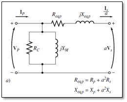
In this section, the math model of electric transformers is shown. This model is the classic representation used for parametric estimation in distribution electric transformers [10]. The represented model is developed in real variable,which can be implemented and verified using an optimization tool such as GAMS or AMPL [15]. Fig. 1 represents a single-phase transformer and its circuit representation-called the equivalent circuit model.

Hence, the electric transformer is represented using the following elements: primary coil series branch with resistance and reactance; parallel branch with conductance and susceptance (magnetization branch); the transformation ratio (α); and the secondary coil series branch with resistance and reactance [15]. They are described as follows:
Resistance and reactance of the primary coil series branch (RP + jXP); RP models active power loss in the primary coil, and XP represents the reactive power and leakage flux.
Magnetization branch (RC||jXM). RC models the power loss at the core of the transformer; XM represents the energy associated with the effort made to magnetize the magnetic domains at the ferromagnetic core.
The transformation ratio (a): This ratio is built using an adequate number of coil turns relations between primary and secondary coils. It determines the variation of the voltage level from the primary side to the secondary side.
Resistance and reactance of the secondary coil series branch (RS + jXS), RS models active power loss in the primary coil, and XS signifies the reactive power and leakage flux in the secondary coil.
With the aim of reducing parameters to be estimated, all the series elements were referred to the primary side, and then the values of resistance and inductance were simplified to single values (R eqP + jX eqP ). Also, the magnetization branch was moved to the source side; it is possible that the current in the parallel branch is small enough to allow the changes proposed [15].
In Fig. 2, Isp is the secondary current referred to the primary side with the value
 In the same way, the secondary voltage referred to the primary side is Vsp=aVs. With this reduced circuit, we can perform an analysis using Kirchhoff laws.
Source: Authors.
Figure 2 Equivalent model of the single-phase transformer. Parameters on the primary side.
Now, with the aforementioned discussion, we can establish that the parametric estimation problem entails how the parameters of ReqP, XeqP, RC, and XM can be determined by using current and voltage of the actual transformers to be studied.
Then, for the approach, we propose an objective function considering the quadratic mean error to be minimized in the procedure. The objective function in Z is composed by voltages and currents measured from the transformer according to [24]. This is presented in Eq. (1).

In Eq. (1),
 denote the electric current and voltages measured. Also, the symbol |x| is the magnitude of the complex variable x.The set of constraints in this problem is presented in Eqs. (2) a (9).


Here, variables A and B are as follows: 𝐴=


In the above equations, Xmax and Xmin are the upper and lower limits for the decision variables. Those variables are the parameters ReqP, XeqP, RC, and XM in Fig. 2.
The math model in Eqs. (1) to (9) can be interpreted as follows: Eq. (1) is the objective function that has been built from the quadratic mean error between the measures and estimation. The expected minimum for Z is zero, as the estimated variables have values close to the real measured variables. Eq. (2) contains the calculations of load current on the primary side of the transformer by using the transformer parameters; this is obtained by applying Kirchhoff’s law to the external loop of the equivalent circuit. Eq. (3) that indicates the source current is obtained by applying Kirchhoff’s first law in the node in which both series equivalent and parallel branches are connected. This could be understood as the sum of the magnetization current and the current of the load referred to primary coil (Isp). Eq. (4) determines the output voltage applied to the load; in this case, the load is considered mainly resistive-inductive (RL) as is typical among end users. Expressions (5)-(8) are the constraints for the values, but they must be understood as the space of solutions for the decision variables (parameters of the electric transformer). Now, the estimated values are at the level of ohms, while the magnetization values are at the level of thousands of ohms [10]. Finally, Eq. (9) demonstrates the relation between the resistance and the reactance of the transformer coil. It is certain that those values are typically inductive.
3.Methodology for the parametric estimation
The optimization model that allows for the obtaining of the parameters of the electric transformer is nonlinear and usually classified as a problem of nonlinear programming (NLP). This is described by the set of Eqs. (1)-(9). To solve this problem, we propose a numeric method indicating good results in this kind of problems. The combinatorial optimization technique used here is the sine-cosine algorithm (SCA).
The SCA is a metaheuristic optimization tool powerful for continuous problems with nonlinearities and non-convexities [25]. The method could be classified into the family of evolutionary algorithms, and its evolution is based on trigonometric functions and their combinations, which gives the name to the method [26]. Some of the most relevant works in the literature review are the following: the optimal power flow in distribution and transmission systems [27], parametric estimation in photovoltaic systems [26], minimization in nonlinear functions [28], and tuning of parameters in machine learning algorithms [29].
3.1 Generation of the initial population
The SCA, like all evolutionary algorithms, is a searching algorithm that find solutions (each solution is an individual, and a group of individuals corresponds to the population), and they change at each iteration (generation of population). The algorithm runs until it reaches a good solution after some iterations. Hence, the algorithm begins the search from an initial population. The population in each generation generates offspring by introducing changes to the individual’s phenotype. These changes may be introduced by crossover, the mutation of an individual, or another strategy. The changes allow for a new individual (solutions), which can explore the space of solutions until reaching a good solution [25]. A solution is a candidate to be a good solution if its value of Z is as good as the best solution kept from the other previous generation. Now, the initial population is represented as follows [26]:

where n denotes the number of variables in the problem; in the parametric estimation problem of the distribution transformer, the number of parameters is four, so n=4. For the same matrix in Eq. (10), P is the number of individuals selected to create the population; this is, the number of candidate solutions. Here, the matrix X0 corresponds to the initial population at 0 iteration. For the specific case of the problem faced here, the variables in the matrix can be understood as follows: Xj1 represents solutions for the parameter Rc, Xj2 signifies values for Reqp, Xj3 represents the variable XM, and Xj4 denotes the variable Xeqp.
One the main features of the SCA is the evolution of population with individuals (solutions) contained in the space of solutions (this implies feasibility). This feature is usually avoided in genetic algorithms. In this sense, the constraints (5)-(8) are considered to create the initial population, as presented in Eq. (11) [26]:

Here, i corresponds to the row and j corresponds to the column of the matrix X0, and r1 is a random number with normal distribution in the rank [0,1]. Now, Xj max and Xj min denote the maximum and minimum values for the variables.
3.2 Fitness function
The offspring of the population in evolutionary algorithms is intrinsically random, because the new generation of population is obtained by the mutation of individuals and by crossover of them. It produces infeasible solutions, which can eventually offer new phenotypes to the population to reach new zones with a possible better solution in further iterations [27]. In this paper, we take advantage of this idea while forcefully keeping the new individuals in the feasible space. This was made using the following adaptation function such as the function in Eq. in (1):

Here, γ is a penalty factor that force solutions to move from the infeasibility zone to the feasibility space along the evolution of the population. This value is always positive to increase the penalty for deviations; we used γ=100 according to the suggestions in [26]. Now, when all the sets of constraints are accomplished by the solution, the value of the component {0,Xeqp- βReqp} is zero; hence, values from Eq. (12) and (1) are the same [27]. Lastly, the set of the constraints (5)-(8) have always accomplished even since the initial iteration 0, because the first population is created using Eq. (11).
3.2.1 Evolution of the population
The evolution here uses a rule based on trigonometric functions; in this way, it explores the space of solutions to find good candidates [30]. To apply this criterion, all the solutions in the initial population X0 are evaluated, then the best solution is selected and called Xbest.Thereafter, Xbest is used to obtain yt+1 or xt+1, as illustrated in Eq. (13) [27].


In Eqs. (13) and (14), r3 y r4 are also random numbers with normal distribution in the rank [0,1] and [-π, -π] respectively [25].Moreover, r2 is a factor with variations that play an important role in the convergence of the algorithm. This value changes according with Eq. (15), reducing its value while increasing the number of iterations. In the equation, tmáx is the maximum number of iterations considered for the SCA optimization process [27].

In the algorithm, the individuals Yi t+1 and Zi t+1 can be part of the population in new generations, usually replacing an older individual Xi t. Following are the three criteria to follow while making this substitution [30].
Set Xi t+1= Yi t+1 as the candidate solution if Zf (Yi t+1)< Zf (Zi t), and if it is better than Zf (Xi t+1).
Set Xi t+1= Zi t+1 as the candidate solution if Zf (Zi t+1)< Zf (Yi t), and if it is better than Zf (Xi t+1).
Otherwise, set Xi t+1= Xi t. This is done when the individual has no changes from one generation to the other.
It is important to mention that before evaluating the individuals Yi t+1 and Zi t+1 in the adaptation function (12), they must be adjusted using Eq. (11) to preserve the feasibility of the population.
3.2.2 Stop criteria for the algorithm
The SCA iterative process ends according to the following conditions [25]:
3.2.3 Algorithm
The computational implementation of the SCA for the parametric estimation in electric transformers is summed up using the Algorithm 1 [27].

4 Test cases
This section will consider three test systems having an equal number of electric transformers with typical nominal values according to the standards of manufacturers and power systems in Colombia [15].
4.1 Test case 1
The first test case is a single-phase transformer with the following features: 20 kVA, 8000/240 V, and 60 Hz, with β greater than 3 [10]. Table 1 indicates that the electric transformer operates in normal conditions with a resistive load. This implies that XL=0.Moreover, Table 2 presents the maximum and minimum values for the parameters.


4.2 Test case 2
The second test case corresponds to a single-phase transformer having the features 45 kVA, 11400/240 V y 60 Hz, with β= 4.5. Table 3 presents all the electrical parameters for this test system and Table 4 indicates the maximum and minimum bounds of the decision variables.


4.3 Test case 3
The third test case is a single-phase transformer with the following features: 112.5 kVA, 13200/440 V y, and 60 Hz.
In this case, the load has an inductive component. The electric transformer feeds a load with an inductive power factor of 0.8666. Table 5 shows all the electrical parameters for this test system and Table 6 presents the lower and upper bounds of the decision variables.


5 Computational validation
For the purpose of the SCA implementation, Algorithm A was implemented. It was made using MATLAB® 2015. The simulations were run on a PC with the following features: Intel® Core™ i3-4005U CPU @ 1.70GHz. RAM 4Gb, Windows 10 64-bit. Regarding the parametric information of the SCA, we selected 100000 iterations with a population of 100 individuals. The parameters were tuned after multiple simulations. Note that these parameters for the SCA have been tuned after multiple simulations that considered populations sizes from 50 to 150 as well as iterations between 30000 to 120000 to determine the best performance between the optimal solution and the total processing times.
5.1 Results for the test case 1
Table 7 shows the results from the SCA implemented using MATLAB®. It took around 302.67 seconds to find the optimal solution.

Table 7 depicts the objective as Zf=7.11E-13, which can be considered zero. Therefore, this could be considered the optimal solution. After 100 iterations, the results obtained were a little better than those obtained using GAMS and reported in [15]. The results in [15] were obtained using an objective function with a value for the objective function of Z=2.64053E-11.
Related to the parametric values, the value for the magnetization resistance is 164564.9598 Ω, and the real value is 159000 Ω. The error is close to 3.5%. The value for the magnetization reactance is 36736.37 Ω, and the actual value is 38400 Ω. The error here is around 4.33%. The value for the series resistance is 38.0717 Ω, and the real value is 38.4 Ω. The error here is lower than the previous parameters with 0.85%. Finally, the value for the series reactance is 197.4227 Ω, and the actual value is 192 Ω. The error here is 2.82%. In the series parameters (important for power losses studies and voltage regulation), the errors were in general low.
5.2 Test case 2
Table 8 shows the results after running the SCA on MATLAB®. A computational time of 300.5030 seconds was taken to find the optimal solution.

From Table 8, we can see that the objective function takes a value of Zf=3.61649E-12.This practically has a value of zero, and the result obtained can be considered the optimal solution for the problem. After 100 iterations, even the first five iterations produced better results than those reported in [15] using GAMS. In the paper used for comparison purposes, the objective function reached a value of Z =2.36872E-11.
Regarding the parametric values, in Case 2, the value for the magnetization resistance is 245676.21 Ω, and the real value is 220000 Ω. The error is 11.67%. The value for the magnetization reactance is 45541.33 Ω, and the actual value is 64500 Ω. The error here is 29.39%. The value for the series resistance is 47.7173 Ω, and the real value is 45 Ω. The error here is lower than in the parallel branch-6.04%. Finally, the value for the series reactance is 160.32 Ω, and the actual value is 204 Ω. The error here is 21.41%. In this case, the errors were greater than that in Test case 1.
5.3 Test case 3
Table 9 exhibits the results obtained after a computational time of 307.9022 s. This case is simulated by considering an inductive load with a power factor of 0.8666.

The objective function value in this case takes the value Zf=4.74464E-13.As in the previous cases, this value can be interpreted as zero, which implies the reaching of the optimal solution, since the first iterations in the SCA offered better solutions than those reported in [15] and obtained using GAMS software. In the work reviewed, the objective function took a value for Z=1.25467E-12.
Now, the parametric values found by the SCA are as follows: the value for the magnetization resistance is 200344.44 Ω, and the real value is 252440 Ω. For this parameter, the estimation error is 20.64%. Next, the value of the magnetization reactance is 99450.44 Ω, and the real value is 68712 Ω. For this branch component, the error is 44.74%. Moreover, for the series components, the series resistance takes a value of 55.23 Ω, with a real value of 48.5 Ω. Consequently, the error for this parameter is 13.88%. Lastly, the series reactance takes the value 151.27 Ω Ω, and the real value reported is 210.8 Ω, which implies an error of 28.24%. Even with small values for the objective function, there are errors between estimated parameters and real parameters.
A review of the errors allows us to establish that bigger errors emerge in the estimation of the magnetization branch with 4.33%, 29.39%, and 44.74% for Case 1, 2, and 3 respectively. Those big errors could be provoked due to the nonlinear nature of the optimization problem, which is built with roots, divisions, and complex functions. Its highly nonlinear nature can create multiple possibilities to reduce the objective function to zero even with deviations in the estimated parameters. Fortunately, the magnetization branch has a small effect on the total model, as the parameters have big values and therefore the current flowing through the parallel component is tiny. In the nominal load for distribution transformers, this contribution can be neglected.
5.4 Comparisons between real values and estimated values
In this subsection, we have proposed an additional computational experiment to establish the differences between the estimated parameters and the real parameters reported. In the test, a simulation of an electric transformer was run to feed an electric demand. In this way, it was possible to make some comparisons. In this case, we employed the data for the Test case 3.
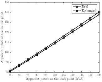
The electric transformer in the simulation was used to feed a power load in the rank of 75-125 kVA, considering a power-lagging power factor of 0.90. It is worth mentioning that in the simulations, the real case was run using the parameters suggested by the manufacturer on the nameplate of the transformer. However, it is possible that these parameters could suffer some alterations depending on how long the transformer is being used. Figs. 3 and 4 are present the apparent power input and the efficiency calculation of the real and estimate models of the transformer. For simplicity in the simulation, we assume that the voltage at the source terminals is maintained in the nominal operative conditions, i.e., 13.2 kV.
Results in Figs. 3 and 4 show that the estimated model follows the behavior of the ideal parameters of the transformer with average calculation errors of about 1.46 % in the case of the apparent power inputs, and 0.07 % in the case of the efficiency calculation. These results allow us to conclude that the parametric estimation approach based on the SCA using voltage and current measures is efficient to determine the electrical parameters of the single-phase transformers, since the global error behavior in the worst estimation case was lower than 2 %. This behavior was good even with the high difference between the parameters on the nameplate of the transformer and the estimated values. In addition, these results confirm that due to the nonlinear non-convex characteristics of the optimization model, multiple combinations of the parameters can exist, which guarantee an adequate electrical performance of the transformer.

6 Conclusions and future works
This paper has addressed the problem of parametric estimation in single-phase transformers using voltage and current measures by implementing the sine-cosine algorithm. The SCA is a math-inspired optimization approach that allows for exploring and exploiting the solution space by using trigonometric evaluation rules. Numerical results demonstrated that lower objective function values were reached with the SCA in comparison with the GAMS approach, with the main advantage that multiple solutions were found with adequate objective function performances, i.e., 1E-11,in all the simulation cases.
Numerical results also showed that the parameter with the most difference compared with the real value was the magnetizing reactance across all the test systems; however, due to their values in the order of thousands of ohms connected in parallel to the voltage source made this parameter have a low influence on the global performance of the transformer. This was verified in underload transformer simulations in which the error between the apparent power input with real and estimated parameters in the worst scenario (see the third test system) was lower than the 2 %.
In terms of future works, it will be possible to conduct the following researches: (i) the application of the recent developed optimization algorithms such the vortex search algorithm and the crow search algorithm to estimate the parameters in single-phase transformers due the promissory results recently reported by these algorithms in parametric estimation problems; and (ii) the inclusion of the series branch on the primary side of the model of the transformer to disaggregate the effect of active and reactive power losses in both windings of the transformer.

