Introduction
To determine the stress-strain states generated within embankments due to applied loads and gravity, researchers have developed analytical and empirical methods (Lamas et al., 2011; Standing et al., 2020) that enable the design and enforcement of the project within the admissible parameters of durability and deformability. Moreover, modelling techniques have been used to develop constitutive models (Feng et al., 2020; Jiang et al., 2020; Li et al., 2021). So far, in Cuba, there are no available studies, either theoretical or experimental, on construction regulations and standards under different climatic and traffic conditions concerning the performance of slopes, such as the design and construction of the embankments in a highway.
The strength and density levels that must be reached are currently defined through empirical methods by current Cuban standards (NC-11, 2005). This mainly limits the design of embankments of great height because the acting loads exceed the maximum allowed stress. Thus, the need arises for the conception and building of a numerical model to simulate, with admissible error, the stress-strain performance of these embankment fundamentals in highway projects. Additionally, this contributes to improving the current official design and construction standards.
Several numerical methods can be used to calculate the stress-strain state of a structure: boundary elements, finite volumes, finite differences, and the finite-element method, among others (Haftka and Malkus, 1981; Namdar, 2020; Osipov etal., 2018; Otalvaro and Nanclares, 2009). This study uses the finite-element method, which, conceptually, is the breakdown of a continuous physical element into a discrete number of parts or elements that are connected by a number of points called nodes. The movements of these are the main variables to calculate in each problem (Anderson et al., 2021; Zienkiewicz etal., 2015). Within each element, the movements of any point are determined from the movements of the nodes of each element using inverse or semi-inverse formulations (Álvarez, 2014).
One of the fundamental advantages of using the finite-element method in these problems is the reduction of experimental costs once the model is properly represented. However, the numerical model must be calibrated and validated. In this study, two calibration procedures are performed: one by applying the error theory, and the other by using non-parametric hypothesis tests. The results of the plate-load test have been used to validate this procedure.
Overview from embankment construction and design
For a continuous circulation of traffic on highways, with quality and safety during the period of use, embankments must meet certain requirements regarding stability, safety, and strength under the forces exerted by weather and traffic (Mesa, 2017).
Experience in construction embankments has enabled us to prepare firm structures under favorable conditions in terms of topography and materials. However, for problematic conditions, considering the nature of the materials, as well as for geomorphology, many authors have indicated the need to take special safety measures, thus requiring the development of independent projects for each case, given that those are special cases that require further study. For example, Huang et al., (2010) used a two-dimensional finite method to investigate the stress and strain of embankments built on soft ground, with or without treatment of the foundation. Liu et al. (2004) undertook an experimental study on high embankment construction for an expressway. Stuedlein et al. (2010) presented a 46 m design for a mechanically stabilized earth wall with a fill slope of 2:1 inclination. Ulloa and Vargas (2007) described a methodology to detect the physical vulnerability of fillings and embankments on mountains and slopes. Shan et al. (2009) studied soil compaction, taking into account the performance of an already built high embankment vs. the thaw phenomenon; and Guoxiong et al. (2010) evaluated slope stability through 2D and 3D analysis in high embankments. Murata et al. (2020) evaluated pavement and embankments by means of a superficial technique. Although, in recent years, many of the studies for road embankments only focus on pavement and the first layers of the base and subbase (Albarazi, 2020; Hernandez-López et al., 2020), others focus on deformational state behavior (Mesa et al., 2020; Pardo de Santayana et al., 2020).
Soil, unlike any other material, has an extremely complex behavior, which is dependent on its type, the in situ treatment received, the compaction level, the state of aggregation, etc. Therefore, many countries have developed several criteria for characterizing soils according to their features or the needs of the project (AASHTO, 2021; PG-3, 2017). Approximately 80% of the materials of the embankment constitute the core, in which fine-grained materials can be used, such as clays, silts, and residual soils, if adequate compaction control is carried out, given the potential deformability.
The methods used in practice to estimate settlements are often based on in situ tests, such as the Vane cone test, the Standard penetration test (SPT), and the plate-load test.
The plate-load test can be used as part of a soil inspection procedure for foundations design (ASTM, 1994). It was also developed to study the foundation soil of roads and airports. After being developed and improved, it is currently an essential test for the calculation and subsequent monitoring of civil engineering projects. The test is performed in situ on the soil to measure the vertical settlement due to the applied load. This test consists of applying a vertical load on a circular metal plate that is firmly seated and levelled on the embankment. When the test preparations are verified, different loads are applied, and the load required for different strain rates is calculated (Figure 1) (Anyang et al., 2018; NC-11, 2005; Patel, 2019).
The aim of this study is to demonstrate the calibration procedure of a finite element model by means of the results of different plate-load tests applied to embankments constructed (physical model) within the project of the refinery plant built in the province of Cienfuegos, Cuba. Data concerning displacements and loads were used to validate the numerical models of the embankment.
Different constitutive models have been used for soil modeling. These models differ from each other in the parameters used for the calculation (e.g. responses such as elastic-plastic, energy dissipation, permanent deformations, etc.) (Zhang etal., 2021). Examples of constitutive models include elastic models, elastic-plastic models, or those based on the critical state.
Elastic models show a linear relationship between applied stresses and deformations, where the instant of applying tension coincides with the moment that the soil deformation ends. These models clearly do not simulate soil performance in an adequate way, since they do not consider residual deformations. However, for the sake of simplicity, they are useful for modeling the initial stress states of embankments. Elastic-plastic models consider the elastic and plastic states of the material. When the remaining deformation is considered, and hence the stress and displacements are reached in soil structures, it is possible to predict their behavior against predetermined load systems. Critical-state models are based on the study of the energy-dissipation mechanisms within the soil skeleton, as well as the observation of the macroscopic behavior of materials.
Incremental hypoelastic models establish a relationship between stress application velocity and strain velocity using a tensorial function. Since this requires a large number of parameters and demanding computer-memory capabilities when integrated into finite-element programs, it has not had significant practical applications. The Kondner-Duncan model, which establishes a hyperbolic function that causes serious continuity problems, was one of the first models adapted to simulate the behavior of large masses of soil such as dam fronts (Mellah et al., 2000).
Hyperbolic models easily represent the stress-strain behavior for the drained-soil response. The model was initially proposed by Kondner and Zelasko (1963) and was subsequently presented on an incremental basis by Duncan and Chan (1970). It assumes that the stress-strain curves of soil can approximate a hyperbola (Lamas et al., 2011).
From all the models mentioned above, the elastic-plastic Mohr-Coulomb model was chosen for this research because the parameters used are readily available, it is best adapted to the behavior of the soil, and it may reach the maximum load break with values between 400 and 500 kPa (Gu et al., 2020; Hai-Sui, 2006; Nieto etal., 2009). The Mohr-Coulomb criterion assumes that failure occurs when the shear stress at any point in a material reaches a value that depends linearly on the normal stress on the same plane. This model is based on Mohr's circle for states of stress at failure on the plane of the maximum and minimum principal stresses. The break line is the common tangent to all Mohr circles.
Therefore, the Mohr-Coulomb model is defined by Equation (1), where a is negative in compression, from the average of the maximum and minimum Mohr's circle; c is the cohesion; ø the friction angle; σ m the principal stresses; and S is half the difference between the maximum and minimum principal stresses.
Where τ = S cos ∅; σ = σm + S sin ∅τ (kPa), c (kPa) , σ (kPa), ∅ (◦), S (kPa) , σm (kPa)
For general states of stress, it is more convenient to write the model in terms of three stress invariants, as shown in Equation (2) (Abaqus/CAE, 2017).
Where θ is the deviatory polar angle defined (o); q is the Mises equivalent stress (kPa); p is the equivalent pressure stress (kPa); r is the third invariant deviatory stress (kPa); and S is the deviatory stress (kPa).
Study area: geotechnical and geological framework
The embankments used for the validation tests are in areas occupied by the facilities of the Camilo Cienfuegos oil refinery. According to the coordinates of the Lambert conical projection system, they are in northern Cuba, from 548450 to 550500 and from 261 000 to 264 300. Its height ranges between 0,00 m to 40,00 m, as reported by the National Altimetry System. They are located in the region of Siboney, Industrial Zone No. 3 ("Carolina") of the city of Cienfuegos in the Republic of Cuba (Figure 2). This refinery is a project of the National Applied Research Company (ENIA) and an Invescons Research Unit construction. In geomorphological terms, the territory was originally a semi-wavy, cumulative-abrasive-denudative marine terrace, and it currently has a slightly rugged topography. It is a product of the human earth movements made for the construction of the refinery between 1995 and 2005.
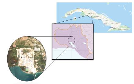
Source: Authors, based on the report courtesy of Cienfuegos's ENIA.
Figure 2 Camilo Cienfuegos oil refinery area.
The area is located within the neo-autochthonous basin of the Palaeocene-Quaternary depression of Cienfuegos, on its north-western flank. The geological structure of the territory consists of pyroclastic-carbonate, terrigenous-carbonate, and carbonate sedimentary rocks from the Upper Cretaceous, Palaeocene, and Neogene of the Cantabria, Caunao and Paso Real formations, in addition to different Quaternary materials, undifferentiated as formations. Almost all of the faults that complicate the formations in pre-Eocene flanks dissipate towards the inside of the depression, with no seismogenic faults in the environment.
With the parameters determined from embankment testing conducted in the city of Cienfuegos (Figure 2), it is possible to correctly simulate soil behavior using numerical methods. It is also possible to simulate the plate-load test, which was chosen for validation and subsequent use in determining the deformation and strength of soils.
Materials and tests
In this study, the data calculated from the drilling with UGB-50 bits by ENIA project was used. The methods used in the drilling were percussion and/or rotation due to the soil type. The determination of the index properties was performed according to specifications of international standards group (ASTM, 2000).
The geotechnical profile was characterized to a depth of 29 m. From the samples taken, the parameters of the existing soils in the area were calculated. Tables 1 and 2 show their values.
Table 1 Index properties of the soils
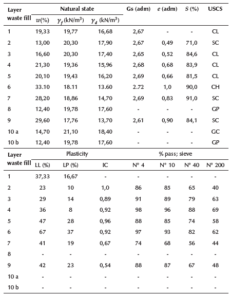
Note: Where: w natural humidity; yf natural volumetric specific weigh; yd dry volumetric specific weight; Gs relative specific weight of solids; e void ratio; S saturation; USCS Unified Soil Classification System; LL Liquid limit; LP Plastic limit; IC Consistency Index; No 4, No 10, No 40 and No 200 sieve size according to ASTM (2000); USCS column Unified Soil Classification System from ASTM (2000); CL Lean clay; SC Clayey sand; CH Fat clay; GP Poorly graded gravel; GC Clayey gravel.
Source: Adapted from technical report, courtesy of Cienfuegos's ENIA.
Table 2 Physical-mechanical properties of the soils
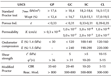
Source: Adapted from technical report, courtesy of Cienfuegos's ENIA.
These tables indicate that the foundation soil, down to 10 m deep, consists of interstratified soils of sandy-clay type with medium to low plasticity and a mean natural density of 19,6 KN/m3, with a standard deviation of 0,68. Furthermore, the soil has an average natural moisture of 20,7% that has somewhat higher dispersion values (between 13 and 33%).
Regarding the values of the mechanical parameters used in the calculations, the effective cohesion has a mean value of 12,0 KPa, with a maximum of 15,0 kPa and a minimum of 5 kPa; and the angle of effective internal friction averaged 15 degrees (a maximum of 20o and a minimum of 10o).
In the project, three test polygons were executed, each one for 30 plate-load tests. This study was conducted to characterize the zone through a geological engineering investigation on the feasibility of the refinery expansion.
For the characterization of the landfill of the embankment in the polygons, the index properties were determined, and 24 direct shear tests were performed according to Cuban standards (NC-325, 2004), as well as an Oedometer test (Table 3).
Table 3 Physical-mechanical properties of the soil fill

Source: Adapted from technical report Courtesy of Cienfuegos's ENIA.
The most representative results from the plate-load tests are shown in Figure 3. The mean value of the most representative tests of the polygons is presented in Table 4. It can be observed that the data of polygon number 2 are not representative of the entire set, which is why this polygon has not been used in the calibration process.
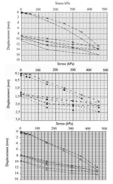
Source: Authors/Adapted from technical report, courtesy of Cienfuegos's ENIA.
Figure 3 Load-plate test results from: a) polygon 1, b) polygon 2, c) polygon 3.
Numerical model
The invariants of the modelling process (geometry, loads, materials, and boundary conditions) were taken into account to elaborate a model that corresponded with the real study.
The geometry of the model was performed in accordance with the existing polygons in terms of height, slope gradient, and crown width. Figure 4 shows the average dimensions of polygons and deep layers of soil.
The distance from the toe of the slope to the boundary condition was established from previous studies to determine the subdomain model (Mesa et al., 2016). The analysis of the influence of stress in the area of crown and core of previous studies determined that the distance most useful for modeling road embankments is eight times the ratio of the base of the slope and height of the embankment,. Linear bonds are used as the boundary condition (Figure 4) (Mesa et al., 2016).
The thicknesses of the underlying soil were considered for the depth of the sample perforations performed; the results are in accordance with the physical-mechanical properties found in the laboratory.
The constitutive model used, Mohr-Coulomb, is well suited for soil behavior at breakage; it stands out over the others because the parameters can be determined from laboratory tests. Regarding the system of loads, stresses applied according to the test at different stages of construction were used (Mesa, et al., 2016). The numerical model of this study is limited to a plane strain model.
Calibration of the mathematical model
From the preparation of the mathematical model of this paper, two important variables were defined: the type of finite element (TFE) and the optimal discretization of domain (DD).
Geo-Studio 2012 was used for this study. This software has different TFE, and only three were used, as shown in Figure 5. For the selection of the mathematical model, a 23 test design was defined, varying the two parameters (TFE and DD) at three levels each: 50 cm, 100 cm, and 125 cm; and quadrilateral with four-node, quadrilateral with eight-node and triangular with three-node, respectively (Figure 5) (Mesa, 2017).
Table 5 Expressions to compute the errors at one and several points
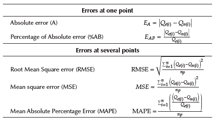
Note: Where: (Q e(i))Control pattern results; (Q (i)) Results obtained from the numerical model; tip Analysis points.
Source: Adapted from Mesa and Alvarez (2011).
Nine simulations were performed with the conditions of Figure 4, varying the TFE and DD as shown in Figure 5. After the simulations were completed, an analysis of the results was made. The theory of errors (Table 5) (Kaizhong and Shiyong, 2019) was employed. The errors at several points were applied for each model.
Table 5 shows two expressions used for errors at one point and, three expressions used for several points. All expressions depend on the results of the control pattern (Q e(i)), that is, the results obtained from the experimental test and the results from the numerical model (Q n(i)).
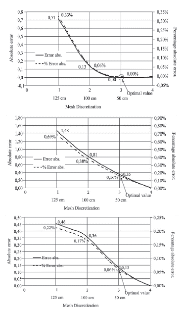
Figure 6 shows the results from the errors at one point. These are from previous research conducted by the authors (Mesa and Álvarez, 2011). In that study, it was found that the TFE of the quadrilateral 4-node with a discretization of the domain of 50 cm is the mathematical model that best explains the stress-strain results on road embankments, since 8-node elements show greater errors (Figure 6b). Based on these results, the finite element quadrilateral of 4-node and triangular with 3-node were combined in this work (Figure 7).
Source: Authors, based on the results from Mesa and Álvarez (2011).
Figure 6 Absolute and percentage of absolute errors in one point with: a) quadrilateral 4-node, b) quadrilateral 8-node, c) triangular 3-node.
Another way to calibrate the model is by using statistics. In order to compare the results from the model and the experimental tests and determine the similarity or difference between results, a parametric or non-parametric test must be carried out.
It is known that, for comparing and determining similarities between two independent samples, it is necessary to perform a parametric (t-student) or non-parametric (Mann-Whitney U) test. The parametric test is applicable if the samples fit a normal distribution and their variance is homogeneous. Otherwise, non-parametric tests should be applied for the comparison (Figure 8).
First, a normality Kolmogorov-Smirnov (K-S) test was applied to determine if the samples fit a normal distribution. The null hypothesis (H0) assumption was that the samples fit a distribution, and, as an alternative hypothesis (H1), the negation of H0. Additionally, the homogeneity of variance test from Levene was applied.
Results
The problem was simulated with the data shown above, recreating the plate-load test in the process of loading and unloading for a given period of time (Table 6).
Table 6 Values of the loading and unloading process

Source: Adapted from technical report, courtesy of Cienfuegos's ENIA.
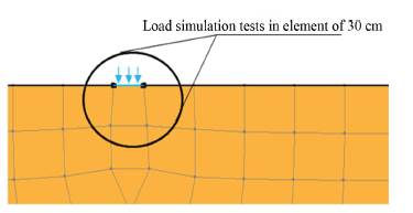
The geometry of the foundation soil was defined considering the stratification and, after simulating the initial stress, the load of the 3 m high embankment was added. Later stages of implementation regarding the loading and unloading for each of the pressures determined in the test and the application time of the load were defined. For the simulation, the test area with 30 cm elements was zoned to represent the circular plate of 300 mm in diameter and a distributed load on the element equal to the test value (Figure 9).
Source: Authors
Figure 9 Zoom-in of the simulation of the load-plate test on the finite element size of 30 cm.
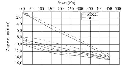
After the test was modeled, the results of the soil strain by the load system were represented graphically as stress-displacement curves for both the model and the test (Figure 10).
Source: Authors
Figure 10 Stress-displacement curves from model and average of results from polygon 3.
From the results of polygons 1 and 3, the average was obtained and graphically represented as shown in Figure 10. The RMSE, MSE, and MAPE from Table 5 were applied to the results from polygons 1 and 3, since the data of polygon number 2 was not representative.
The MSE and RMSE was 0,49 and 0,70, respectively, for polygon 3; and, for polygon 1, the results were 2,49 and 1,58, respectively. Chai and Draxler (2014) suggest that RMSE is a better metric to present the results than MAE. The error in those cases was 0,70 and 1,58 for polygons 3 and 1, respectively. On the other hand, the value of the MAPE was 9 and 12% for polygons 3 and 1, respectively. It should be noted that, in engineering, acceptable errors are between 5 and 10%. As there are many variables involved in this process and some imprecision in measurements or parameters from the literature, a 12% of error was accepted.
However, this paper presents another way to calibrate the numerical model through the determination of similarities between two independent samples by means of statistical hypotheses. Table 7 shows the K-S test for polygons and the model, where no data fits the normal distribution, since the P-value was less than 0,05.
On the other hand, the Levene test was applied with the null hypothesis that the population variances are equal. As is shown in Table 8, the P-value was higher than 0,05 when the model was compared with polygons 1 and 3, thus corroborating the similarities in variances. The P-value of polygon 2 was less than 0,05, thus corroborating that those experiments were not representative.
Then, as the data did not fit a normal distribution, a non-parametric Mann-Whitney U test was used, under the assumption of the null hypothesis (H0) that the samples have statistically similar median, as well as an alternative hypothesis (H1): the negation of H0 that the medians of samples are not similar. The test was applied with a confidence level of 95%. This means that, if the P-value is greater than 0,05, the samples have a similar median.
The results in Table 9 show that the significance level was higher than 0,05 for polygons 1 and 3, and thus the null hypothesis was not rejected, which indicates that the samples (model and experimental) can be considered similar. This result matches previously reported results when considering the error theory (9 and 12% for polygons 3 and 1, respectively). Therefore, it is confirmed that the results from the model and those from the load-plate tests (from polygons 1 and 3) were similar.
Conclusions
In this paper, the simulation of a load-plate test was performed by using the numerical method of finite elements, based on the project report of the National Applied Research Company (ENIA) of Cuba. An overview of the constitutive models to be applied in soil was carried out. Additionally, to calibrate the numerical model, two procedures were followed: using the error theory and performing the non-parametric hypothesis statistical test of Mann-Whitney U. For both procedures, the results from the model and the experimental data are similar. Moreover, the results show that a load-plate test can be modeled using FEM. To reproduce other load plate tests by using the finite element model, it is necessary to provide the geotechnical characteristics, geometry, and geomorphology of the soils. The procedures shown in this paper can be used in other studies related to soil calibration problems where experimental data are available.


