


 English (pdf)
 Article in xml format
 Article references
 Send this article by e-mail
 Cited by SciELO
  Cited by Google
  Similars in
SciELO
Similars in
SciELO  Similars in Google
 Permalink
I. INTRODUCTION
Rock slope stability is a significant concern in mining and infrastructure projects. However, predicting the mechanical response of a fracture rock mass when subjected to a loading process is a complex task since the response is highly controlled by the interactions among blocks, which geometry is defined by the presence of discontinuities.
The conventional practice deals with complexity by grouping the complex and uncertain geometry of rock blocks within the rock mass into well-defined failure mechanics with an explicit pre-defined geometry. Accordingly, the well-known planar, wedge, and toppling failure kinematic controlled mechanisms of failure are analyzed by limit equilibrium. Such an assessment is reduced to deterministic models based on mean planes and slope orientation. This approach disregards both the aleatory and epistemic uncertainty; the former is associated with the natural variability of joints orientation, and the latter to the limitations of the measuring technique to understand the rock mass discontinuities geometry comprehensively.
Despite the simplifications linked to the kinematically controlled mechanisms, the wedge failures model considers the tetrahedron formed by two discontinuity planes, an upper slope, and the main slope. This tridimensional representation of the rock blocks allows to consider the variability of the orientation of two joint sets within an explicit limit equilibrium formulation in terms of the factor of safety (FS). The stability assessment of wedges implies the formulation of equilibrium of forces in a three-dimensional space. This problem has been solved by stereographic projections [1] [2].
However, when a reliability assessment is performed, an explicit solution is more suitable because several realizations of the model must be computed. Low [3] developed a closed-form equation without graphical assistance based on a geometric interpretation of the wedge. Subsequently, [4], [5] extended the equation to an inclined upper slope. This solution has been applied to perform wedge failure reliability assessment [4], [6], [7]. Moreover, Low’s model has also been used to estimate system’s probability of rock wedges by conditional probability-based methods [8]. The latter work takes advantage of the wedge model flexibility to implement its methodology in a spreadsheet. Other solutions have been applied to perform a probabilistic analysis of wedges [9], [10] - [12] including directional statistics.
A general approach using three-dimensional vector algebra was developed by [13], which is a widely used solution implemented in the Swedge commercial software (available at www.rocscience.com). Former implementations of this approach were developed by [14] and [15]; the deterministic model was extended to perform a probabilistic analysis of those wedges. This solution has been implemented along with the Barton-Bandis failure criterion to perform reliability back analysis of rock wedges [16] and system reliability seismic pseudo-static with the same failure criterion [17].
Another limit equilibrium approach implemented along with a nonlinear strength criterion has been proposed by [18]. This criterion involves the assumption of the shear forces on both sides of the slip surface, which is not considered by the Mohr-Coulomb and the Barton-Bandis failure criteria. However, this approach has not been extended to the probabilistic analysis yet.
Within this framework, we conducted a probabilistic analysis of rock wedges and performed a level III probabilistic analysis by a Monte Carlo simulation. This analysis resorts to Low’s model but introduces an algorithm to identify the modes of failure systematically. Besides, information on rock slopes is taken using a close-range stereoscopy technique, which gathers more robust data sets on joint orientations. Finally, the proposed algorithms were implemented into a program coded in Python.
II. MATERIALS AND METHODS
A. Deterministic Wedge Stability Model
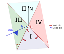
Figure 1 shows the geometry of a potentially unstable wedge. The model can analyze four modes of failure in this sort of wedges: failure along the intersection of both joint planes, failure along either joint plane 1 or plane 2, and lifting failure.

The wedge’s factor of safety is computed according to Equation 1, when the failure occurs along the intersection line.
where, Φ1 and Φ2 are the friction angles of planes 1 and 2, respectively. 𝑐1 and 𝑐2 correspond to the cohesion of planes 1 and 2. 𝐺𝑤 is the water pressure coefficient of a pyramidal distribution. ℎ is the slope height, and H is the total height, including the upper slope. 𝑎1, 𝑎2, 𝑏1, and 𝑏2 are geometric coefficients which are a function of the following angles:
𝜍1 is the horizontal angle between the strike line of plane 1 and the line of intersection between the upper ground surface and the slope face. Idem for 𝜍2 in plane 2. In this model the modes of failure are related to these angles (Figure 2). 𝛿1 and 𝛿2 are the dip angle of planes 1 and 2, respectively.

Equation 1 may be straightforwardly programmable. However, it resorts to horizontal angles 𝜍1, 𝜍2, 𝛿1 and 𝛿2,, which cannot be computed explicitly from the wedge geometry. Low [5] presents a graphical approach to compute these angles, based on the strikes of joint and slope planes, and applies the model to a wedge that fails along the intersection line. However, there is no reference to a systematic way to compute those horizontal angles, which is crucial since they define the mode of failure.
Moreover, even though relative joint slope orientations lead to a given mode of failure, e.g., along plane 2, when the variability of joints orientation is considered in the probabilistic analysis, it is likely to have orientation combinations that yield other failure mode.
Accordingly, this work evaluates a broad range of possible combinations of joint and slope planes considering the planes as a Fisher-distributed random variable. Hence, different failure modes are expected (along intersection lines, plane 1, plane 2, or lost on contact). Moreover, thousands of realizations of the model are carried out.
B. Algorithm to Define the Mode of Failure
An algorithm to compute angles 𝜍1, 𝜍2, 𝛿1 and 𝛿2 is proposed in this section. It is based on the trend of the planes as depicted in Figure 3. These trend lines are treated as vectors to generate a fixed set-up, which allows defining the corresponding mode of failure.

The first step is to generate a reference set-up of planes, which applies to all possible relative orientations of input planes. The procedure proposed to find this arrangement is the following:
Define two horizontal vectors dd i (plunge = 0) oriented as the dip direction, 𝛼𝑖, of joint planes:
1. Define the horizontal vector t i and express it according to their direction cosines:
2. Order the joint planes so that the third component of the cross product is positive. This condition guarantees a unique order assignation for joint planes.
4. Then, considering that planes are vectors rather than axis, give a convenient definition of the orientation of joint planes (𝜄1,𝜄2), and the slope (𝜄𝑠)
With the described algorithm, a set-up such as the one plotted in Figure 3 is obtained. Here, the angle between joint planes is always less than 180°, which generates four regions where the slope line,
Region I: Wedge slides along plane 1. 𝜄𝑠 lies in this region if 𝜄1< 𝜄𝑠<𝜄2
Region II: Wedge slides along plane 2. 𝜄𝑠 lies in this region if 𝜄1+180 < 𝜄𝑠<𝜄2+180
Region III: Wedge slides along intersection of planes. 𝜄𝑠 lies in this region if 𝜄1< 𝜄𝑠<𝜄2+180
Region IV: No sliding wedge is formed. 𝜄𝑠 lies in this region if 𝜄2+180< 𝜄𝑠<𝜄1.
Once identifying within which region 𝜄𝑠 falls, angles 𝜍1, 𝜍2, 𝛿1 and 𝛿2 are calculated. This task requires some additional refinement depending on what quadrants 𝜄1,𝜄2 are located. As an example, the results for 0≤ 𝜄1<180 and 0≤ 𝜄2<180 are presented below.
1. If
If
If
This process is repeated for every combination of
C. Fisher Distribution
The orientation of planes within a joint set is modeled as a Fisher distributed random variable to account for their variability. The Fisher is a unimodal rotational symmetric distribution around a true orientation [20]. Hence, the distribution is represented by three parameters, i.e., the dip, 𝛽, and the dip direction 𝛼 of the mean orientation, as well as a concentration parameter 𝜅. The latter represents the variability around the mean orientation: the larger 𝜅, the larger the dispersion of the data.
In this work, the distribution parameters 𝛼,𝛽 and 𝜅 of each joint set were estimated from the measured planes. Then, several orientation planes are generated by a Monte Carlo simulation. A detailed explanation of the parameters estimation and planes simulation is presented in [20], [21].
D. Removable and Unstable Blocks
The block presented in Section 2.1 is a removable block resulting from the intersection of two joint planes and two slope planes. However, not every combination yields a potentially unstable wedge. Hence, a kinematic analysis was carried out to verify if the block is removable before checking the block stability. The conditions for a block to be removable are [22]:
D. Reliability Assessment Methods
Reliability assessment methods can be classified as follows, depending on the type of calculation [23]
Level I: At this level no failure probabilities are calculated. The design is performed under standards.
Level II: At this level, the probability of failure is calculated by linearizing the reliability function in a carefully selected point.
Level III: Methods at this level compute the probability of failure considering the probability density function of all strength and load variables.
In this work, a Monte Carlo procedure was selected, which belongs to level III reliability methods.
E. Probability of Failure
To perform the probabilistic analysis, the joint orientation was considered as a random variable that represents the aleatory uncertainty inherent to the orientation of joints. This random variable was assumed to follow a Fisher distribution.
As for the analysis, joint strength parameters were considered deterministic, as well as slope trend and plunge.
The procedure to compute the probability of failure of rock wedges by a Monte Carlo simulation is the following:
Define joint sets by a k-means clustering algorithm.
Compute the Fisher distribution parameters for each joint set.
Simulate a joint orientation for each joint set by a Monte Carlo simulation. For the i th simulation of the two joint planes:
a. Verify the kinematic conditions for removability. If not removable, go back to step 2. If kinematically unstable, update the number of removable blocks, 𝑁𝑟𝑒𝑚𝑜𝑣𝑎𝑏𝑙𝑒:
𝑁𝑟𝑒𝑚𝑜𝑣𝑎𝑏𝑙𝑒=𝑁𝑟𝑒𝑚𝑜𝑣𝑎𝑏𝑙𝑒+1
b. Compute the factor of safety (FS) according to Equation 1. If FS<1.0, update the number of unstable blocks, 𝑁𝑢𝑛𝑠𝑡𝑎𝑏𝑙𝑒:
𝑁𝑢𝑛𝑠𝑡𝑎𝑏𝑙𝑒=𝑁𝑢𝑛𝑠𝑡𝑎𝑏𝑙𝑒+1
4. Simulate the i th +1 combination of joint planes.
5. To repeat while 𝑖<𝑁, where N is the desired number of realizations of the model.
As a result, the factor of safety of each realization is obtained, along with the number of removable and unstable blocks. Consequently, the probability of failure (PF) can be computed as follows:
From these results, a probability function can be built for the removable blocks since the total cumulative probability must be equal to 1.
III. RESULTS
The algorithm proposed in this work was applied to the structural information collected in a sandstone mine located in Une, Cundinamarca. The quarry exploits a sedimentary rock mass that consists of interbedded layers of claystone and sandstone, as shown in Figure 5. A detailed presentation on the geology and structural information of the quarry is presented in [24], [25].

Figure 6 summarizes the structural information collected in the mine in 2017 using a short-range stereoscopy system [25]. This information was clustered by a K-means algorithm yielding the joint sets reported in Table 1, with their corresponding mean orientation and concentration parameters and assuming that they follow a Fisher distribution. There are three joint sets (red and green), two subvertical and one bedding plane (blue).

Table 1 Joint sets statistical parameters.
| Joint set 1 | Joint set 2 | Bedding | |
|---|---|---|---|
| Number of poles (N) | 826 | 743 | 593 |
| Dip direction (°) | 171.1 | 51.9 | 294.4 |
| Dip (°) | 85.8 | 79.8 | 14.4 |
As for the other parameters, they were assumed as deterministic as follows:
Slope dip direction = 330° and 89°
Slope inclination = 70°
Upper slope angle = 10°
Slope height = 15m
Geomechanical parameters were taken from shear tests along joints as follows:
Stability analysis was performed for wedges formed by:
For these planes, the assessed values of
The first task is to validate the results obtained by the algorithm proposed in section 2.2. Hence, stability analyses were performed by this algorithm and compared to the results yielded by the commercial software. Some selected results are included in Table 2. As can be seen, results obtained with the proposed algorithm match those yielded by Swedge. This validation is critical since the Monte Carlo simulation requires thousands of FS computations.
Table 2 Wedge FS computed by the proposed algorithm and Swedge.
| Realization | FS by the proposed algorithm | FS computed by Swedge | Realization | FS by the proposed algorithm | FS computed by Swedge |
|---|---|---|---|---|---|
| 1 | 1.4 | 1.4 | 9 | 2.5 | 2.5 |
| 2 | 1.5 | 1.5 | 10 | 2.6 | 2.6 |
| 3 | 0.8 | 0.8 | 11 | 1.6 | 1.6 |
| 4 | 0.9 | 0.9 | 12 | 1.7 | 1.7 |
| 5 | 1.1 | 1.1 | 13 | 2.1 | 2.1 |
| 6 | 1.0 | 1.0 | 14 | 1.9 | 1.9 |
| 7 | 1.1 | 1.1 | 15 | 2.0 | 2.0 |
| 8 | 1.1 | 1.1 |
Once the algorithm is validated, the next step is simulating the planes’ orientations for stability analysis. According to the statistical parameters reported in Table 1, 50,000 planes were simulated from each joint set. Figure 7 depicts stereonets with the simulated planes of each joint set with
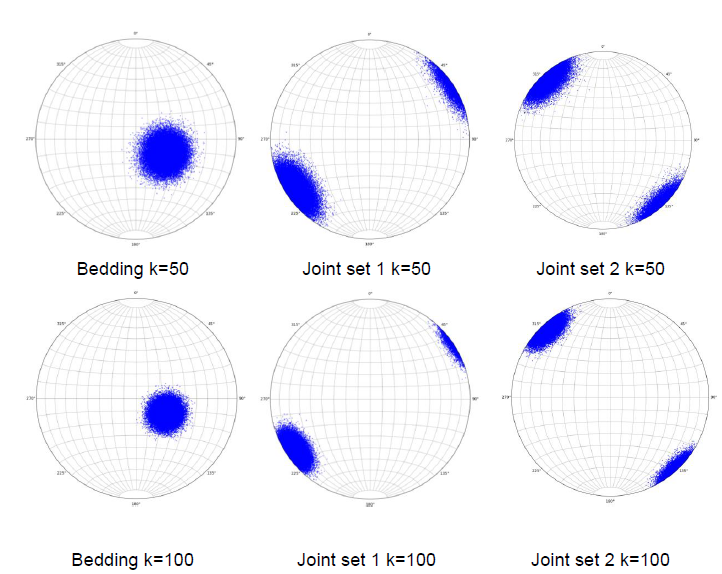
Fig. 7 Factor of safety probability functions of removable blocks formed by bedding and joint set 1.
Subsequently, with the simulated planes, the factor of safety was computed 50,000 times for each
Table 3 Probability of failure of the wedge formed by bedding and joint set 1.
| Concentration parameter, κ | Bedding - Joint 1 (Wedge 1) | Joint 1- Joint 2 (Wedge 2) |
|---|---|---|
| Probability of failure | Probability of failure | |
| 10 | 0.04895 | 0.18250 |
| 20 | 0.01402 | 0.16872 |
| 50 | 0.00028 | 0.07352 |
| 100 | 0.00000 | 0.05516 |
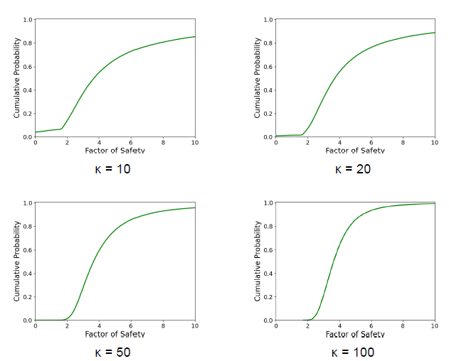
Fig. 8 Factor of safety probability functions of removable blocks formed by bedding and joint set 1 (Wedge 1).
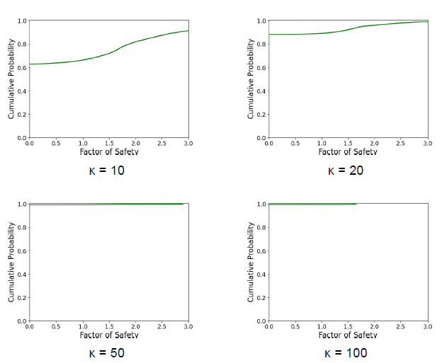
Fig. 9 Factor of safety probability functions of removable blocks formed by bedding and joint set 1 (Wedge 2).
The first noticeable result is that the probability of failure reported in Table 3 is smaller than the one included in figures 8 and 9. This is because the probability of failure is computed using the total number of realizations of the model, while the probability function is built with the removable blocks. This is the result of performing a kinematic analysis before the kinetic stability assessment.
This result highlights the importance of considering the total number of simulations to compute the probability of failure, not only the removable blocks, since the combination of planes that lead to nonremovable blocks is also likely. If they are not considered, the probability of failure is overestimated.
On the other hand, there is a reduction in the probability of failure as
The probability functions also provide information on the failure modes, even for the same set of planes. For instance, for wedge 1, as
IV. CONCLUSIONS
This paper presents a reliability assessment of rock wedges by Monte Carlo simulation. An algorithm based on joints and slope planes trend vectorial analysis is proposed to define the modes of failure and it was incorporated within a limit equilibrium wedge stability model. This algorithm is the main contribution of this work. The algorithm was coded in Python and compared to a commercial software to validated it.
Besides, the reliability analysis involves a kinematic analysis to define the removable block prior to the latter to assess the wedge stability. Therefore, the total number of realizations of the analysis should be considered to compute the probability of failure; otherwise, this probability is overestimated.
The reliability analysis showed the importance of accounting for the variability of joint orientation; if not, several likely combinations of joint orientation with a more critical stability condition than the yielded by the mean orientation are disregarded. Unfortunately, there is no way to consider those critical wedges by a deterministic analysis.
We suggest further analysis considering rotational nonsymmetric distributions to model the variability of joint sets orientation to get a more accurate description and more reliable results on the probability of failure.

