INTRODUCTION
State contracting is a relevant issue for society because it is through this mechanism that State resources are invested. Each time a public entity initiates a process to acquire goods or services, it creates a public procurement market that allows for competition among the bidders, as long as plurality is guaranteed [1]. Similarly, the selection of the contractor and the bidding method represent vital steps in the acquisition process of the project [2-4]. In Colombia, state contracts are regulated by Law 80 of 1993, which lays down rules and principles governing the contracts of state entities, including the enabling requirements of financial capacity that must be met by bidders [5]. The Colombian Society of Engineers (SCI) conducts the Study of the Regional Public Contracting of Colombia, which analyzes the plurality of the bidders of the contracting processes that are awarded, alerting that more than 60 % of the contracting processes are tendered with less than three bidders, identifying this problem as a national phenomenon that must be remedied [6]. A warning on the possibilities of corruption that threatens State resources is identified [7] by pointing out the factors related to the enabling requirements of financial capacity in the draft specifications, which do not guarantee the plurality of bidders, specifically in the segment of the Electronic System for Public Procurement - (SECOP) called Land, Buildings, Structures and Roads. The insufficient, inefficient, and unsustainable provision of infrastructure, which characterizes the Latin American region, represents one of the factors preventing progress towards sustainable development. One of the causes of the scarcity and low quality of infrastructure is the low levels of public investment in the sector and the gap between investment and need [8].
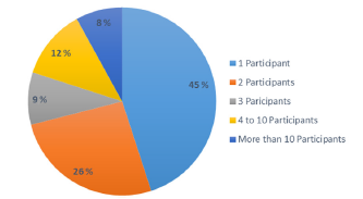
The SCI in the "Regional Public Procurement Study" conducted in 2017 exposes the problems related to irregularities in public procurement processes, with special emphasis on the lack of plurality of bidders [9]. It is evident that 81 % of the awarded contracts have between one and three bidders, which reinforces the aforementioned problem, as can be seen in Figure 1.

Source: own elaboration.
Figure 1 Percentage of Contracts according to number of proponents - Public Bidding
The financial capacity indicators make it possible to establish minimum conditions reflecting the financial situation of the tenderers through liquidity and indebtedness, with the aim of ensuring that the tenderer complies fully and on time with the purpose of the contract [10].
The evaluation of the Current Ratio (CR) considers that if the result is equal or greater than 1, it implies acceptable liquidity. However, a high current ratio only benefits creditors and may not necessarily be the company; that is, it is not justifiable to have a high cash flow or high level of stock but little productivity, due to the opportunity cost [11]. According to the theoretical explanation, inversely proportional behavior was expected in the proposed model. That is, the higher the liquidity index required, the lower the probability of the proponents complying, that is, the lower the probability of plurality in the process. The equation (1) shows the mathematical expression for the Current Ratio.
Debt Index (DI): Determines the degree of indebtedness in the financing structure (liabilities and equity) of the proposer. The higher the debt ratio, the greater is the likelihood that the proposer will not meet its liabilities [10]. These indicators allow us to know the degree of participation of creditors in the financing of the company, measure the total percentage of funds coming from credits, and understand the result as the percentage of assets that have been financed by debt or liabilities [12], [13]. According to the theoretical explanation, directly proportional behavior is expected. That is to say, the higher the debt index required, the greater the probability of proponents complying with this requirement, resulting in a higher likelihood of plurality in the process. The equation for Debt Index is shown in (2).
Interest Coverage Ratio (ICR): Reflects the proposer's ability to meet financial obligations. The higher the interest coverage, the less likely the bidder is to default on its financial obligations [10]. The formula for the calculation is as follows: it allows to identify how the operating profit covers interests generated by liabilities, that is, the number of times the company covers interests with operating profit [14]. Because of the theoretical explanation, an inversely proportional behavior is expected; that is, the higher the interest coverage ratio, the lower is the probability of bidders' plurality. Equation (3) shows the mathematical calculation of Interest Coverage Ratio.
1. RESEARCH METHOD
The methodology used for the development of this research includes several steps. Firstly, with the objective of analyzing the information deposited in the SECOP in 2017, a representative statistical sample of the study population was established, keeping in mind the random selection criteria as a Simple Random Sample, guaranteeing that all the individuals that make up the population have the same probability of being included [15], using the equation (4).
Where:
Z: Constant that depends on the confidence level obtained by means of the standard normal distribution table N (0,1)
N: Total number of cases/observations/population
p: Proportion of individuals in the population with the study characteristic
q: Proportion of individuals who do not possess, in the population, the characteristic of study
e: Desired sample error
n: Optimal sample size
Then, based on the equation presented above, the calculation of the sample needed to proceed with the analysis of the 2017 tenders was made and is shown in Table 1.
Table 1 Status of the Tenders.
| Status | Processes in SECOP | Sample Processes |
|---|---|---|
| Call for proposals | 31 | 29 |
| Adjudicated | 181 | 135 |
| Held | 590 | 242 |
| Abnormally terminated after call | 52 | 46 |
Source: own elaboration.
For each tender, the variables being studied are the following: the department where the process is executed; Status, Amount, Group in the SECOP, Segment in SECOP, Family in SECOP, Class at SECOP, Liquidity rate required in the draft specification; debt ratio required in the draft specifications; reason for coverage required in the draft specification; number of observations submitted by proposers for each of the indices measuring the financial standing requirement, number of proposers who submitted comments on the draft terms of reference in relation to the financial capacity requirements, number of proponents in each bidding process, number of proponents determined skilled in each bidding process, and number of proposers determined to be unfit for business due to non-compliance with financial capacity requirements for each tender process.
Based on the information collected, a binary statistical model is proposed that allows the estimation of the probability of occurrence of a phenomenon from the study variables, ensuring that the result is in the range of 0 to 1, following the behavior of the logistic distribution function. Initially, the variables mentioned are considered, with the objective of knowing the probability of occurrence of a bidding process that does not have a plurality of bidders. Based on the weights that will be established for each of the variables of the binary statistical model, the impact of enabling requirements of financial capacity on the number of skilled bidders in public tenders under study will be identified.
1.1. Binary statistical model
Statistical analysis of data with dichotomous variables or variables measured in ordinal and nominal scales is frequently performed. Particularly in binary models, the response variable has two possible results, called success and failure, which are represented by 0 and 1. For the specific development of the proposed model, the response variable assumes two possible values[16]:
- 0 when the tender process does not have a plurality of bidders
- 1 when the bidding process has a plurality of bidders, that is, 2 or more bidders presented themselves to the process
This corresponds to arbitrary assignments for a qualitative response [17]. The binary regression is characterized by having a qualitative dependent variable with two values that configure the presence or absence of a certain characteristic; for the present investigation, the presence or absence of a plurality of bidders in the bidding processes will be determined [18]. For a binary choice model to be fully specified, it is necessary to know the F function on which it is defined, which allows two types of models to be analyzed, as shown in the equation (5) and (6) :
• Logistics Distribution (Logit Statistical Model)
• Standard Normal Distribution (Probit Model)
1.1.1 Logit statistical model
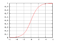
The Logit statistical model is similar to the traditional regression with the main difference being the logistic and non-linear estimation function, generating as a result the probability estimate that a sample individual belongs to a particular group [16], [19], [20]. This model allows the response variable to be qualitative in order to know the probability of an event occurring, i.e. the variable is binary or dichotomous [21]. Identifying the model that best defines the behavior of the variables is possible by comparing the models proposed using the likelihood coefficient, which allows us to identify from the data extracted from the sample how much more probable a model is compared to another [20]. Due to the binary behavior of the response variable, there is empirical evidence that indicates the form that the response function should take; a monotonously increasing S-shaped function [17] such as that observed in the Figure 2.
The process of formulating and analysing the Logit regression model must take into account the following aspects shown in Table 2.
Table 2 Analysis Process - Logit Model
| Selection of the Model Variables | Definition of an analysis model to justify a dependency model |
| Analysis of application conditions | |
| Identify the relationship of each independent variable to the dependent variable | |
| Analyze the relationships between the independent variables to establish possible co-linearity situations | |
| Consider the inclusion of interactions | |
| Follow a process of selection of the best variables in order to adjust the best model [18]. | |
| Estimation of the coefficients of the independent variables | Application of a maximum likelihood estimation method, a case of Ordinary Square Minima (OSM) |
| The coefficients assess the importance of each independent variable, quantitative (with a single value), qualitative (establishing a reference category and generating one or more coefficients) and possible interactions [18]. | |
| Model Evaluation | The aim is to establish the model’s goodness of fit or explanatory capacity |
| The predictive efficiency or discriminating capacity of the model; arises from the crossing of the dependent variable observed by the predicted | |
| Analysis of the extreme values by means of an analysis of the residues, detecting influential cases, analysing measures of influence and multicollinearity. | |
| Interpretation of the results with all the information, but fundamentally giving an account of the table of coefficients [18]. |
Source: own elaboration.
The R software presents a programming environment consisting of a set of tools that facilitate the statistical analysis of data. The use of R has increased in recent years from academic and research environments to enterprise production environments [22]. Initially, the outliers in the study sample were analyzed by normalizing the values of the dependent variables, which allowed the analysis of the distance in terms of standard deviations that a point is found with respect to the reference mean, establishing -3 as the lower limit and +3 as the upper limit. Tenders whose standardization was lower than -3 or higher than 3.The following procedure is performed to analyze each of the independent variables:
The average of the values recorded in the tenders under study is calculated.
The standard deviation of the values under study is calculated.
The normalization of the data is performed using the normalization function that evaluates the normalized value of a distribution characterized by a mean and standard deviation, as shown in equation (7):
2. RESULTS AND DISCUSSIONS
In this study, a binomial logistic model is fitted, the model seeks to include the independent variables, Interest coverage ratio, Debt ratio, Current Ratio, Observations. Only variables that are directly related to the financial capacity indicators that are required in the specifications as enabling requirements are considered for the model approach. The method of choosing variables backwards is proposed for the design of the other models, that is, eliminating the variable that is not significant in this model. For each proposed model, the Akaike - AIC information criteria are analyzed, which provides a simple and objective method to select the most appropriate one that characterizes the experimental data, providing an estimate of the distance between the model and the mechanism that generates the observed data. The AIC criteria formulate the problem of model selection as a search for the model that presents the lowest AIC value among a set of candidate models, looking for a model that loses the least amount of information [23]. The AIC criteria values for the three models are presented in Table 3. The model 2 has the lowest AIC; the supports and validations on which this model is chosen for forecasting, as well as the independent variables that compose it, will be shown below.
Table 3 Akaike Information Criteria for the models.
| Model | AIC Criteria |
|---|---|
| Model 1 | 358,8964 |
| Model 2 | 356,9811 |
| Model 3 | 358,1768 |
Source: own elaboration.
2.1. Developed model
According to the AIC criteria, the second model is selected as the most accurated of the tested models, in this case, the debt variable is discarded, and the following variables are included: Interest coverage ratio, Current Ratio, Observations. The coefficients and probability values for each variable were estimated with the same levels of significance as mentioned above. Here, the intercept is discarded because it does not comply with this parameter, it is showed in Table 4. The equation 8 is proposed for Model 2:
Table 4 Result R - Coefficients Model 2
| Coefficients | |||||
|---|---|---|---|---|---|
| Estimate | Std. Error | Z Value | Pr (>|z|) | ||
| (Intercept) | -0.29270 | 0.20457 | -1.431 | 0.15250 | |
| Interest Coverage Ratio - ICR | -0.11552 | 0.03576 | -3.230 | 0.00124 ** | |
| Current Ratio- CR | -0.10516 | 0.04031 | -2.609 | 0.00909 ** | |
| Observations - Obs | 0.18604 | 0.10222 | 1.820 | 0.06878 . | |
| Signif. Codes: 0 ‘***’ 0.001 ‘**’ 0.01 ‘*’ 0.05 ‘.’ | |||||
Source: own elaboration.
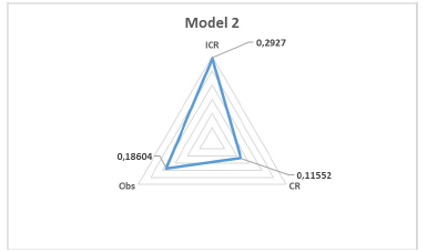
The behavior of the variables of the model is based on what is expected; the increase in one unit of the interest coverage ratio and the current ratio generates a reduction in the probability of bidders' plurality in the bidding processes. In contrast, an increase in one unit of the number of observations increases the probability of a plurality of bidders, as shown in Figure 3.
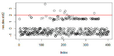
The adjustment level of the values predicted by the model was then checked against the observed values. The standard deviation of the residuals is a measure of goodness of fit that is used to measure the degree of alignment of the data points with the real model [24], for which limits are set, as shown in Figure 4.
As can be seen in Figure 4, the majority of the data are grouped within the permitted limits and show a pattern of behavior in which outliers of less than 5 % of the study population are evident. Cook's distance analysis is performed and there is no presence of influential values in the residual, i.e. no observation has a distance greater than 1 so the residuals are stable.
Thus far, the model has met the assumptions made by which cross-validation is performed by the bootstrapping method, based on repeatedly extracting samples from a dataset and adjusting the model of interest for each sample. Cross-validation is applied to estimate the test error associated with a given statistical method to evaluate the performance of the model and to determine appropriate levels of flexibility [25]. The bootstrapping method consists of generating observations from the distribution of the original sample, obtaining in each simulation a sample typically of the same size as the original sample with which the model was formulated [26]. One of the main uses of this method is the internal validation of regression models, which has the advantage that for the construction of the model, it uses all available data evidencing the sensitivity of the model to changes, which allows us to obtain robust regression equations [27]. The model was analyzed using the bootstrapping and cross-validation method, verifying that the model was 78.7 % accurate. Additionally, the average probability of the process having multiple providers is 20.6 %, which is in accordance with the qualitative analysis of the data presented.
To check the number of observations that were correctly predicted, a matrix or table of confusion was made (Table 5), which is a contingency table that serves as a statistical tool for the analysis of observations, and is a set of values that counts the degree of similarity between paired observations, that is, a set of predicted data and a set of reference data referencia [28]. The diagonal of the confounding matrix shows that 317 data points met the prediction, which confirms the accuracy of the model by 78.7%, as shown in Table 5. Likewise, the adjusted probability of the model of the existence of plurality is measured, indicating that 14.86 % of the processes have a plurality of providers, which supports the validity of the model, as it is a value close to that observed in the qualitative review of the data.
2.1.1 Other tested models
On the other hand, we have fitted the other two models: Model 1 is comprehended by all the theoretical variables considered for this study, and Model 2, which only includes the interest coverage ratio and Current Ratio. We proceeded to estimate the coefficients and probability values for each of the variables in models one and number three, with significance levels between 0.05 and 0.1, as shown in Table 6. In light of the above parameters, for Model 1, the intercept and index of indebtedness are discarded because they do not meet the desired significance level. In Model 3, the intercept is discarded because it does not comply with the desired value at the significance level.
Table 6 Result R - Coefficients Model 1 and Model 3
| Coefficients Model 1 | ||||
|---|---|---|---|---|
| Estimate | Std. Error | Z Value | Pr (>|z|) | |
| (Intercept) | -0.31003 | 0.21122 | -1.468 | 0.14214 |
| Interest Coverage Ratio - ICR | -0.11546 | 0.03581 | -3.225 | 0.00126 ** |
| Debt Index -DI | 0.02929 | 0.09147 | 0.320 | 0.74879 |
| Current Ratio- CR | -0.10539 | 0.04041 | -2.608 | 0.00912 ** |
| Observations - Obs | 0.18735 | 0.10237 | 1.830 | 0.06723 . |
| Signif. Codes: 0 ‘***’ 0.001 ‘**’ 0.01 ‘*’ 0.05 ‘.’ | ||||
| Coefficients Model 3 | ||||
| Estimate | Std. Error | Z Value | Pr (>|z|) | |
| (Intercept) | -0.25008 | 0.20129 | -1.242 | 0.21408 |
| Interest Coverage Ratio - ICR | -0.10929 | 0.03476 | -3.144 | 0.00167 ** |
| Current Ratio- CR | -0.08944 | 0.3832 | -2.334 | 0.01958 * |
| Signif. Codes: 0 ‘***’ 0.001 ‘**’ 0.01 ‘*’ 0.05 ‘.’ | ||||
Source: own elaboration.
In addition, multicollinearity of the independent variables within the model was examined. The objective is to obtain values close to 1, which indicates that there is no multicollinearity that reduces the precision of the estimated coefficients [22], as observed in Table 7. In addition, a chi-square adjustment was performed to check whether the model was significant under the binomial distribution because the model did not show linearity or normality.
Table 7 Multicollinearity
| ICR | DI | CR | Obs |
|---|---|---|---|
| 1.182197 | 1.003896 | 1.254336 | 1.135633 |
Source: own elaboration.
After establishing the logistic regression model, the level of fit of the values predicted by the model was checked against the observed values. The deviance associated with a model is based on comparing the log likelihood under the model with that under the saturated model (S). The deviance is then defined as twice the difference between these two log likelihoods [22]. Most of the data are grouped between the permitted limits and present a pattern of behavior where no outliers greater than 5% of the objects observed are evident, which allows the stability of the model to be validated through the residuals [24]. Cook's distance is also analyzed for the residuals, allowing measuring how the estimator vector changes when each of the observations is eliminated. If the value is greater than one, the presence of outliers is checked, invalidating the strength of the residuals to behave according to the binomial distribution [29]. No further verification tests were carried out owing to the value given in the AIC criterion, which is higher than that of model 2. To identify the most relevant information for each of the structured models, Table 8 presents the assumptions on which Model 2 is chosen as a regression and the prediction model is tested.
3. CONCLUSIONS
A detailed analysis of the enabling requirements of financial capacity demanded in the specifications in 2017 was carried out, which seeks to establish minimum conditions that reflect the financial health of the bidders in order to comply with the contracted object in a timely manner, for which a logit statistical model was developed. Once the Logit regression model has been developed, it can be seen that the liquidity index has a negative coefficient, i.e., an impact that is inversely proportional to the probability of plurality in the number of skilled bidders; for each unit of increase in the liquidity index, the probability of plurality of bidders decreases by 0.105.
Additionally, once the regression model has been developed, it can be seen that the interest coverage ratio presents a negative coefficient, that is to say, an impact that is inversely proportional to the number of skilled bidders. The probability of multiple bidders decreases by 0.115 for each unit, which increases the interest coverage ratio. It is observed that the debt index variable was not significant and was therefore not included. In the analysis of the enabling requirements of financial capacity, the observations made by the bidders were extracted from each of the indices mentioned above, having as a variable in the model, the number of total observations presenting a behavior directly proportional to the number of skilled bidders; that is, for each unit that increases the number of observations, the probability of plurality of bidders increases by 0.186.


