Introduction
The effective soil depth (ESD) affects the spatial-temporal hydrological dynamic of soil and plant growth (Tesfa et al., 2009). Approximately 40000 Km2 in the southeastern of Buenos Aires province, region of this study, the ESD is generally limited by the presence of a petrocalcic horizon, locally referred to as "tosca" layer. The tosca usually shows abrupt changes in the thickness, density and depth at very short distances. This complexity determines that conventional methods to describing the spatial pattern of tosca are destructive, expensive and time-consuming. This has limited the precision agriculture spread (Castro Franco et al., 2015). Therefore, there is a need for models with high predictive accuracy of ESD at farm scale, from ancillary information sources ().
Lagacherie (2008), reported the soil science could not be isolated from technological developments in last decades. Actually, these advances have been used to collect ancillary soil information fast, easily and accurately. Furthermore, this information is related to factors of soil formation proposed by Jenny (1941). At this respect, recent go on soil sensors and geomorphometric indices derived from digital elevation models (DEM) have demonstrated high predictive accuracy of the spatial variability in soil properties (Corwin & Lesch, 2003).
It is through the go on sensors that is possible to collect numerous of apparent electrical conductivity (ECa) measurements, in an efficient and cost-effective manner (Friedman, 2005). It has been reported that ECa is influenced by texture, organic matter, soil structure, bulk density and cation exchange capacity (). However, a few studies have reported the tosca effect on ECa (Corwin & Lesch, 2003). Particularly, in the southeastern of Buenos Aires province there is no evidence of studies which use the ECa to modeling the ESD.
The simultaneous use of geomorphometric indices and ECa have improved the spatial prediction of soil properties (Kitchen et al., 2003). It is widely accepted that topography is considered one of the factors which determines the spatial distribution of soil properties. As a result, numerous studies have reported the predictive potential of these indices on the spatial model of soil properties (Lagacherie, 2008). However, there is no evidence about the simultaneous use of geomorphometric indices and ECa to modeling ESD limited by tosca.
The aim of this study was to develop a statistical model that can predict spatial patters of ESD limited by tosca in the southeastern conditions, using both ECa measurements and geomorphometric indices. To get this aim, "Random Forest" algorithm was applied. From our results, we hope to optimize digital soil mapping process at field scale.
Material and methods
Experimental fields
A total of 5 farm fields located in the southeastern of the Buenos Aires province were selected to explore the relationships among effective soil depth and those predictor variables related to factors of soil formation (Figure 1, Table 1). The area studied was 280 hectares. The soils are classified as Typic Argiudoll and Petrocalcic Argiudoll (USDA Taxonomy) ().
Effective soil depth and site variables collection
The ESD up to the tosca layer was the variable to predict. To validating the model efficiency, the ESD was measured in each field. A total of 3035 soil depth measurements were carried out between 2010 and 2012. Each measurement was carried out using a soil hydraulic sampler (Giddings Machine Co., Fort Collins, CO) on a 30-m grid resolution. Table 1, shows the description of site variables.
The numerical calculation of predictor variables was carried out using different geomatic tools. Elevation was measured using a DGPS (Trimble R3 Navigation Limited, USA). A digital elevation model (DEM) was obtained from elevation data. From each DEM, geomorphometric indices were calculated using SAGA-GIS v2.0(tm) Terrain Analysis tool (). The geomorphometric indices were selected according to their capability for representing relief geometry, hydrological features and spatial topographical context in each field. On the one hand, slope and aspect are the primary geomorphometric indices related to basic relief parameters. On the other hand, catchment slope, drainage areas, topographic wetness index (TWI), SAGA wetness index (SWI), stream power index (SPI) and loss soil factor (LS_Factor), are secondary geomorphometric indices related to surface hydrology and spatial topographical context. A detailed description of these algorithms can be found in Hengl & Reuter (2008).
ECa data were collected using Veris 3100(r) (Veris Technologies, Salina, KS, USA). This measurement was carried out in a series of parallel transects spaced 20 m apart (Corwin & Lesch, 2003). The six electrodes configuration is referred to as Wenner array, which is a commonly used on a measurement of soil electrical resistivity (). Veris 3100, have allowed georeference measurements at 0-30 cm (ECa_30) and 0-90 cm (ECa_90), simultaneously.
ESD and predictors were computed with ordinary kriging method using ArcGIS v10. Based on this interpolation, a map was carried out at a spatial resolution of 10 m.
Ensemble of general data set
A dataset was ensemble using all predictors. To facility the comparison among fields, elevation parameter was transformed. The transformation consisted of subtracting at all elevation values, the lowest one for each field. The dataset was prepared as follows: (i) design and confection of a 20 m regular grid for each field, using spatial analyst extension in ArcGis 10.0(tm), (ii) values extraction of variable predictor at each grid point, using the function -extract multi values to point- spatial analyst extension in ArcGIS 10.0.and (iii) unify all points forming the dataset.
The dataset was ensemble using 6145 training dataset, obtained from predictors for all fields. Then, the training dataset was randomly divided into two subsets: a calibration dataset (CD, n=4300) and a validation dataset (VD, n=1845). The CD was used to model the relationship among ESD and predictors, while the VD was used to test the accuracy of the models prediction.
Variable selection and model simplification
A variable selection procedure and the model simplification involved: (i) calibration of "Random Forest" (RF) algorithm, (ii) quantification of the predictors importance, (iii) variables selection and (iv) simplification of predictive model. This procedure is usually used for variable selection in high dimensional issues (Genuer et al., 2010).
The aim of RF calibration is to adjust the parameters of the algorithm in order to develop an optimal predictive model (Guyon & Elisseeff, 2003). This calibration was carried out in two steps. Firstly, correlation among predictors was calculated. Secondly, the parameters of RF were estimated: number of trees in the forest (ntree) and number of predictors evaluated at each node (mtry). The RF calibration procedure was carried out using "RandomForest" library of R v3.1.2. (tm). RF calibrated ntree and mtry parameters using "bootstrap" as method for error estimation (Breiman, 2001). This consists of using several random samples (bootstrap samples) from the CD. Then, RF builds a tree for each bootstrap sample. At each bootstrap sample Xi, one-third of data are left out of it and not used in the construction of the k-th tress, so-called out of bag (out-of-bag (OOB)). OOB estimate of error rate (OOBEER ) is estimated from aggregating trees in the forest. This OOBEER is calculated following equation 1.
Where, yi is the initial ensemble error classification on OOB. As a bootstrap sample is added, an OOB error (yOOB (Xi )) is estimated and repeating k-times. Those mtry and ntree which have the lowest OOBEER should be selected for the model (Breiman, 2001).
The importance classification for predictors was carried out using the procedure known as "permutation accuracy importance". Details are described in Strobl et al. (2009). "permutation accuracy importance" is the most adequate procedure for classifying importance variables when RF is used (Breiman, 2001). Results were graphically represented using "party" R package v3.1.2.
To reduce the number of predictors without losing predictive accuracy, the model is simplified (Xiong et al., 2012). This procedure is running in two steps. First, a prediction model was computed considering all predictors. The purpose was to determine the effect on predictive RF model performance by reducing the number of variables. Second, it was evaluated the RF model simplified with CD and VD.
We used iterative elimination to describe the predictive accuracy of RF model (Xiong et al., 2012). To do this, we used "caret" R package v3.1.2. Coefficient of determination (R2) and Root mean square error (RMSE) for each model were calculated to compare the overall accuracy of RF models while applying iterative elimination. The RF simplified model was applied to estimate the effective soil depth for each field. Then, a regression analysis was carried out among effective soil depth observed and predictive values. This regression was applied to CD and VD. Finally, the prediction performance of RF simplified was compared with a visual analysis of effective soil depth maps generated for each field.
Results and discussion
Table 2, shows mean values and coefficient of variation (CV) for each predictor.
A total of 65% of ESD values were among 75 and 100 cm. Lower ESD means were observed in fields 3 and 4. Ranges of ECa were associated to non-saline soils conditions for all fields (Rhoades, 1996). According to their CV, ECa and ESD seemed to have a similar tendency. Fields 1 and 2, had a lower CV. Both are located in a hill zone, whereas fields 3, 4 and 5 are in a plain area.
Our results suggest that spatial pattern of ESD are complex at field scale. At his respect, Amiotti et al. (2001), reported that complex soil patterns exist at field scale in the southeast of Buenos Aires province. It is due to the soil formation period was characterized up to three different pedogenic cycles. On the other hand, Pazos & Mestelan (2002), demonstrated that complex spatial relationships exist between elevation and ESD up to tosca layer. In general, our results confirm the complexity for tosca spatial pattern at field scale, in all fields studied.
Table 3, shows the properties for each soil map unit and its proportional soil series composition for each field. This information could be used as complement information about understanding the spatial patterns of predictors.
A total of nine soil cartography units are spatially corresponded to experimental fields. General characteristics for each soil series can be found in ). 53% of soil series are Petrocalcic Argiudolls (USDA Taxonomy). The others are Typic Argiudolls. The most important difference between them is the presence or not of petrocalcic horizon, also depth and thickness in the argillic horizon ().
Parameters calibration of " Random Forest " algorithm
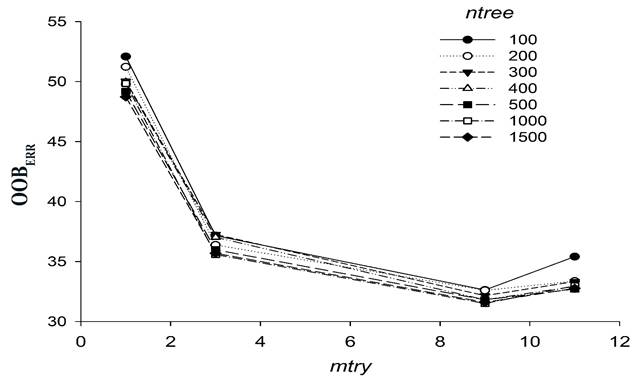
Figure 2, summarizes the simultaneous evaluation OOBEER from mtry and ntree tested. It was evident the effect of mtry increment on OOBEER . When mtry increased, OOBEER decreased from 50% (mtry=1) to 32% (mtry=9). Changes in OOBEER indicate the importance of additional variables. RM model with mtry higher than 9 incremented OOBEER and can generate an over-fit model (Breiman, 2001). The effect of ntree was lower than mtry. RF models with ntree higher than 500 showed more stability.

Figure 2. Relationship between OOBEER and quantity of predictors per node (mtry) for different regression trees (ntree)
In general, our results indicated that mtry equal to 9 and ntree equal to 500 are those parameters of RF model which fit best, in order to achieve an improvement in overall accuracy of ESD.
Predictors importance for effective soil depth
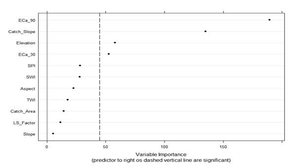
Figure 3, shows the results of "permutation accuracy importance" use.

Figure 3. Predictors importance for effective soil depth data sensitivity to %IncMSE generated by Random Forest algorithm
"Permutation accuracy importance" classifies the variables importance according to difference in prediction before and after a variable was permuted to all ntree. The average of this difference in all ntree, determine the absolute value of predictor importance (Strobl et al., 2009).
Our results suggested that the limit absolute value between relevant and irrelevant variables is 45 (dashed line - Figure 3). According to that, those most important predictors of effective depth were ECa_90, catchment slope, elevation and ECa_30.
Our results showed that ECa could have better predictive accuracy than geomorphometric indices to model ESD. The complexity of spatial pattern of predictors may be related to abrupt changes at short distances for depth, strengthen and thickness in petrocalcic and argillic horizons. According to Dietrich et al. (2014), it is possible that ECa would have affected by: (i) high spatial variability of ESD and (ii) changes in CaCO3 density in the pretrocalcic horizon. Generally, depth tosca present lower CaCO3 density (Pazos & Mestelan, 2002). These changes affect soil hydrological dynamic and thus soil electrical conductance.
Argillic horizon may affect ECa values in mainly two ways. The first, due to the percentage relation between argillic horizon and those underlying and overlying; the second would be attributed to the simultaneous presence of petrocalcic and argillic horizons. This was assessed by Pazos & Mestelan (2002), who reported that the presence of tosca affects either depth and thickness of argillic horizons.
In that context, ECa may possibly be affected by the dynamic of spatial patterns of petrocalcic and argillic horizons. Therefore, ECa can be a potential predictor for determining spatial patterns of ESD.
The importance of catchment slope in the ESD prediction was expectable. This is related to water holding capacity, runoff rate and water drainage (Wilson & Gallant, 2000). It is widely known that these hydrological characteristics are directly related to ESD. Despite that, none evidence was found which had mentioned catchment slope as predictor of ESD. Therefore, this can be a novel result.
Simplification of " Random Forest " model
Figure 4, shows the changes on prediction performance of RF model whereas predictors were iteratively eliminated. That RF model which only uses ECa_90, catchment slope, elevation and ECa_30 had a similar performance as one with all predictors. However, this is not indicating that the rest of predictor lack of prediction accuracy. It would be probably that prediction accuracy could decrease since ECa_90, catchment slope, elevation and ECa_30 had a better prediction performance in the model (Xiong et al., 2012).
Prediction of effective soil depth from simplified model
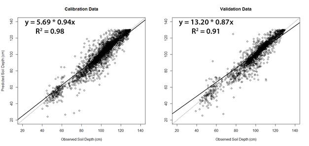
Figure 5, shows the prediction performance of simplified RF model applied to CD and VD. Our results suggested that simplified RF model demonstrated a potential application to ESD prediction. However, its use in others fields is limited for different reasons: (i) a high variability in depth, thickness and CaCO3 density of tosca at short distance, (ii) the relationship between tosca and argillic horizon and (iii) the anthropic effect. It is widely known that the southeast of Buenos Aires province is an outstanding zone due which income depends on agricultural production. Due to that, common suitability land processes such as terraces, crop management zones and drainages had been valuable. Generally, these could affect the spatial pattern of ECa as well as geomorphometric indices and therefore, increase error of simplified RF model developed.

Figure 5. Random Forest model applied for calibration dataset (CD) (R2 = 0.98, P<0.01) and validation dataset (VD) (R2 = 0.91, P<0.01).

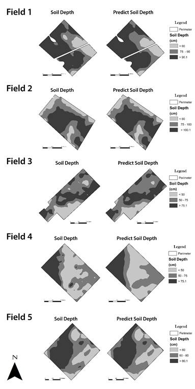
Figure 6. Visual comparison between effective soil depth map and estimated from Random Forest model for all fields
Figure 6, shows maps of effective depth made from simplified RF model development and ESD interpolation. Simplified RF model determined similar spatial patterns of ESD as interpolation technique did. Based on our result, we could validate that RF may be an effective and practical tool to select and predict ESD. However, although this RF model would not have the same performance for all fields, further studies will improve that.
Conclusion
In this study, RF algorithm was used to selecting predictors and developing a simplified model to predict ESD at field scale through soil sensor and geomorphometric indices information. Despite the complexity of tosca spatial patterns, our results show that simplified RF model was an effective and practical tool to predicting spatial patterns of ESD at field scale.
Either tosca and catchment slope are directly correlated to soil hydrological processes and thus could be related to ECa spatial pattern. The RF model which only used ECa_90, catchment slope, elevation and ECa_30 had a similar performance as one considering all predictors. Furthermore, spatial predictions of ESD achieved from simplified RF model were similar to those obtained using interpolation techniques in each field.
RF can be effective to modeling ESD in the southeastern of Buenos Aires condition. However, further studies should be required: (i) to asses relationship among predictors and ESD using a different variable selection method from RF; (ii) to examine specific correlations among ECa, catchment slope and ESD; and (iii) to include others predictors.


