


 English (pdf)
 Article in xml format
 Article references
 Send this article by e-mail
 Cited by SciELO
  Cited by Google
  Similars in
SciELO
Similars in
SciELO  Similars in Google
 Permalink
1. Introduction
Successful mathematical models for tumor growth consider two main stages of development, the stage of free development as an isolated mass of cells, and the vascularized stage, where cells interact with blood an immune cells giving rise to the metastasis process. In the first stage (see for instance [9]) an heterogeneous population of cells is also required for properly model the tumor development. The simplest models consider two kinds of cells within the tumor: on one hand there are quiescent cells that have almost lost their capacity to reproduce and can produce necrosis depending on nutrients, oxygen availability and necrosis substances; on the other hand we consider proliferative cells, which evolve in time increasing their number. The interchange between these two subpopulations can occur by two processes: the recruitment of quiescent tumor cells into proliferative (see [5]) which is supposed to occur at a constant rate; and the inverse process, i.e. the cessation of reproduction for a proliferative cells that changes into quiescent cells at a constant rate.
We consider models for radiation treatment where these tumor cell subpopulations are affected in different ways. Thus proliferative cells may be considered as healthy and quiescent as radiated that is as a sub-product of radiation, as in the terminology of [3], [4]. The passage from healthy into radiated cells occurs at a rate that may be regulated by the radiation treatment. The importance of understanding this models for radiation dosis that evolve in time motivates our work, which may be considered as an extension of the results of [3]. We consider a time, t > 0, dependent T-periodic radiation dosis, D(t) ≥ 0; nevertheless, we consider any continuous function rather than just few representative examples of periodic functions. We conclude the existence of a T-periodic evolution of subpopulations for radiation treatments in Theorem 2.2; we also give sufficient conditions for uniqueness of a stable attracting T-periodic solution in Theorem 2.3.
The tools we use to prove our result arise directly from the Theory of Cooperative systems (see [6, 8]).
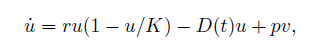
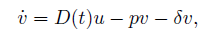
The model consists of the following system of differential equations:
 (1a)
(1a)
 (1b)
(1b)
where (u, v) consists of the pair of healthy (proliferating) and radiated (quiescent) cell subpopulations of the tumor, δ > 0 stands for the constant death rate of radiated cells, 0 < p < 1 stands for the rate of radiated cells that become healthy spontaneously by the process called recruitment of quiescent cells. We consider the logistic growth law for the healthy cells ru(1 − u/K) with r > 0 as the initial grow rate, and K > 0 as the cell capacity (maximal healthy population) which under the supposition of no vascularization remains constant.
2. Results
For the readers convenience we first recall some basic facts about cooperative systems that will be used for proving our results.
For two points ξ, η ∈  denote the partial order ξ ≤ η if ξi ≤ ηi for each i, also denote ξ < η if ξ ≤ η and ξ ̸= v. Consider a system
 (2)
(2)
where f, g are C1 in an open D ⊂  and continuous T-periodic functions on t. System (2) is said a cooperative system in
  × D if
 (3)
(3)
Cooperative systems have very important properties; for a brief introduction to the subject see [8].
We say that a pair of T-periodic differentiable functions (a(t), b(t)) is a sub-solution pair of (2) if
 (4)
(4)
analogously, a pair of T-periodic differentiable functions (A(t), B(t)) is a super-solution pair if
 (5)
(5)
We say that sub- and super-solution pairs are ordered if for all t we have a(t) < A(t) and b(t) < B(t).
An important feature for cooperative system (2) related to periodic orbits was established in [6], Theorem 2.1. Explicitly the following result holds.
Theorem 2.1 (Korman (2016)). Assume that the system (2) is cooperative and has ordered sub- and super-solution pairs (a(t), b(t)) and (A(t), B(t)). Then the system has a T-periodic solution (x(t), y(t)), satisfying a(t) < x(t) < A(t), b(t) < y(t) < B(t), for all t. Furthermore, any solution of (2), with initial condition (x(0), y(0)) satisfying a(0) < x(0) < A(0) and b(0) < y(0) < B(0), converges to the product of the strips
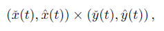
where ( (t),
(t),  (t)),(
 (t),
(t),  (t)) are the minimal, maximal T-periodic solution, respectively.
We complement the previous assertion by saying that there is an implicit assumption, namely that nor x0 ∈ [a(0), A(0)] neither y0 ∈ [b(0), B(0)] exist such that either one or both of the following inequalities hold:
 (6)
(6)
Indeed, if one or both of the equalities (6) hold, then for any initial condition a(0) < x(0) < A(0) and b(0) < y(0) < B(0), the corresponding components of the solution, x(t) or y(t), may converge towards x0 or y0 as t → ∞. Hence, there would exist a solution, (x(t), y(t)), such that  (t) ≡ 0 or
  (t) ≡ 0. Depending on the nature of the system, we could have a locally attractive fixed-point (x0, y0) with a(t) ≤ x0 ≤ A(t) × b(t) ≤ y0 ≤ B(t), instead of a genuine periodic orbit with a(t) < x(t) < A(0), b(0) < y(t) < B(0), ∀t ∈
  .
.
In our situation, the origin is a sub-solution but also a fixed-point solution of system (1). Thus, under certain condition such as (8) in Theorem (2.2) below, there exist a sub-solution super-solution pair (a, b),(A, B) such that a ≡ A ≡ 0 and (0, 0) = (a, b). Therefore, by property (6),

and by substitution we also have  (t) ≡ v0 = 0 ≡
  (t). Therefore, the origin is a local attractive fixed point. Notice that there are no other fixed points for (1).
For the T-periodic continuous function D(t) we set
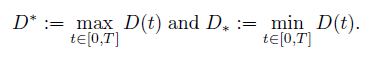 (7)
(7)
Now we state our first result.
Theorem 2.2 (Existence). Assume r, p, δ, K > 0 and D(t) is a non negative, non constant continuous T-periodic function. Then the following mutually exclusive assertions hold.
If
 (8)
(8)
then the origin is a local attractor for every initial condition in a suitable rectangle (u(0), v(0)) ∈ [0, ϵ] × [0, ϵ].
If
 (9)
(9)
then there exists at least one T-periodic solution (u(t), v(t)) of (1) whose components are positive.
Proof. By a straightforward computation the system (1) is cooperative. We construct sub- and super-solution pairs.
For a sub-solution pair; we consider
These functions satisfy the inequalities in (4). Therefore they constitute a sub-solution pair. For constructing a super-solution pair (A(t), B(t)) first we take
 (10)
(10)
with l a positive constant to be chosen.
 (11a)
(11a)
 (11b)
(11b)
Replacing in (5), we get
 (12)
(12)
where
 (13)
(13)
and
 (14)
(14)
We choose B(t) to be the unique positive T-periodic solution of (14); by direct computation we have

with
 (15)
(15)
A short computation shows that
 (16)
(16)
Using (16) and taking into account that D(t) ≥ 0, we have that f′ (l) is bounded above by a quadratic polynomial in l with negative leading term; therefore, there exists l > 0 large enough such that
 (17)
(17)
Thus, considering (17), (12) and (14), we satisfy both inequalities in (5). Consequently, (A(t), B(t)) form a super-solution pair.
Let l0 ≥ −1 be the infimum of the set of values l > −1 such that (17) holds.
When (9) holds, then f ′ (−1) > 0. Moreover, f(−1) = 0 and l0 > −1. For the corresponding supersolution, (A, B), for l > l0, we apply Theorem2.1. Therefore, there exists at least one T-periodic solution for system (1). This proves the second part of the Theorem.
When (8) holds, then f′ (−1) < 0; hence there exists ϵ > 0 such that (17) holds for every l ∈ [−1, −1 + ϵ]. Theorem 2.1 implies that for every l ∈ [−1, −1 + ϵ] and every initial condition (u(0), v(0)) ∈ [0, ϵ] × [0, ϵ 1] with
there exists convergence to a periodic orbit or a fixed point (uϵ(t), vϵ(t)) with a(t) ≤ uϵ(t) ≤ A(t) and b(t) ≤ vϵ(t) ≤ B(t). As ϵ → 0, we have limϵ→0(A, B) = (0, 0); hence, uϵ(t) ≡ 0 ≡ vϵ(t), t ≥ 0. Moreover, l0 = −1 and the origin, (A, B) = (0, 0), is also a super-solution.
This proves the first claim of Theorem 2.2, which proves the result.
Freedman and Pinho in [3] recently investigated the case with perturbed periodic dosage; thus our result presents an alternate proof to its result and extends it. Our existence result Theorem 2.2 naturally raises the questions if the periodic solution is unique and globally attracting.
Recall that a solution (u(t), v(t)) of (2) is globally attracting on a positively invariant set R ⊆  if all solutions (x(t), y(t)) with (x(0), y(0)) ∈ R satisfy
We now establish conditions over the uniqueness and global stability of the periodic solutions.
Theorem 2.3 (Uniqueness). Under condition (9) as in Theorem 2.2, if in addition the following inequality holds,
 (18)
(18)
then there exists a unique T-periodic solution of (1) in  which attracts all other positive solutions as t → ∞. Here
 =
=  D(s) ds.
Under condition (8) as in Theorem 2.2, if (18) holds, then every solution of (1) in  is attracted to the origin as t → ∞.
Proof. Given any periodic T-solution we can chose l > 0 and a solution of (11) with A0 > 0, B0 > 0 large enough, so that we can consider the periodic solution as dominated by this super-solution. According to Theorem 2.1, the set of periodic solutions of (1) is ordered, i.e., we can take the maximal periodic solution, ( (t),
(t),  (t)), as well as the minimal periodic solution, (
 (t),
(t),  (t)), so that for any other periodic solution, (u(t), v(t)), we have
  (t) ≤ u(t) ≤
  (t) and
  (t) ≤ v(t) ≤
  (t). Our strategy is to prove that under condition (18) we actually have (
 (t),
(t),  (t)) = (
 (t),
(t),  (t)).
(t)).
Substitute ( (t),
(t),  (t)) and (
 (t),
(t),  (t)) in (1), then integrate the first equation in (1) over [0, T]. Hence by subtraction we get
integrating the second equation in (1) over [0, T], we obtain

Adding both equations in system (1) and integrating we get
 (19)
(19)
Hence,
Recall that  (t) −
(t) −  (t) ≥ 0; then,

where M ≥ 0 is the supremum of  −
−  . Therefore
  (t) =
(t) =  (t) and by (19) we also have
  (t) =
(t) =  (t).
(t).
We finally use Theorem 2.1 to complete the proof. Indeed, observe that with our construction, by choosing l sufficiently large, we can make the supersolutions arbitrarily large see ((10) and (15)). By the Theorem 2.1, the unique T-periodic solution is then a global attractor for all positive solutions.
3. Examples and applications
In the previous section we established analytically the existence of periodic solutions for system (1) with periodic radiation cancer treatment. The object of this section is to show numerical evidence of the existence of periodic solutions. We numerically solved these equations using Mathematica. The graphs correspond to numerical approximations of the periodic analytic solution. The choice of the parameters arises from empirical data and of actual models and practices from radiotherapy. They should not be taken too seriously if they only show simple plausible applications of our model. The experimental validation of the model and further applications to more subtle model needs to be explored.
For the logistic grow model we take r = 0.502 /day, K = 1297 mm3 , corresponding to the fit of parameters for cells in Lewis lung carcinomas in mice described in [1], with an initial population u(0) + v(0) = 1 units corresponding to 1 mm3 ≈ 106cells.
For the other parameters we refer to the textbook [2]. Here it is explained that the advantages of a multifraction treatment are to spare early reactions on tissues like skin, mucosa, intestinal epitellium in comparison with those that are late responding such as spinal cord. Thus it is important to establish optimal radiation protocols mediating between non-desired effects. We consider an adaptation of the linear-quadratic model (LQ) we have the dose given by D = αd + βd2, where d is the individual dose. Here the biological effective dose (BED) equals

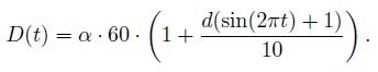
with α ≈ 0.3 the logarithm of cells ‘killed’ per Gy; here we interprete killed as quiescent (see also [10] for this interpretation). Thus, for a Conventional Treatment of 30 fractions α/β = 10/Gy, d = 2 Gy per day. Hence, the periodic discrete dose is specified by D = α · 60 · ( 1 +  ) . If we adapt a continuous dose function, we get
Notice that D ∗ = 18. For δ > 0.002 condition (18) holds.
For the estimation of the parameter p we consider a constant dose per day whose total dose is the proliferation correction of the dose [2]. For the protocol of the conventional treatment this yields p = α(8.3 Gy/30 days) = 0.083.
Example 3.1. For the two initial subpopulations we consider the growth fraction (GF) estimated as 0.5; which is the midpoint of the experimental range 0.3 ∼ 0.7 in certain mice carcinoma. Thus for a GF value of 0.5 we have u(0) = 0.5, v(0) = 0.5; δ may be estimated from an experimental rate denominated ‘cell-loss factor’ (ϕ) described in textbook [2]. Thus take δ = 0.7 as the cell-killing factor arising only by necrosis in quiescent cells in mouse carcinome. Thus the system (1) becomes
 (20a)
(20a)
 (20b)
(20b)
(see Fig. 1).
Numerical evidence, using Mathematica, supports the claim that the tumor vanishes for sufficiently long time (see Fig. 2). Actually (8) holds, therefore the origin is a local attractor as stated in the first claim in Theorem 2.2. Here condition (18) also holds, therefore the origin is a global attractor.

Figure 1. Time plots for sub-population u(t) for δ = 0.7. We observe that the solutions for several initial conditions: (u(0), v(0)) ∈ {(0.5, 0.5), (5, 0), (0, 0.5)} vanish.

Figure 2. Phase space plots for u(t), v(t) with δ = 0.7 and initial conditions (u(0), v(0)) ∈ {(0.5, 0.5), (5, 0), (0, 0.5)}. There is a scaling factor of 10−2 for the u component.
The following examples are motivated by natural questions about the conditions for existence and stability. The choice for the parameters do not arise from experimental data. Related results and models can be seen in [7], where periodic function coefficients are considered and other criteria are described. It would be interesting to find the full picture, with a precise description of all different dynamics that may appear in this model.
Example 3.2. Take δ0 = rp/(D∗ − r) = 0.0024098. Neither condition (8) nor condition (9) hold, therefore we can not claim that certain initial conditions converge either to the origin or to a periodic orbit. Actually orbits seem to converge towards different ω−limit sets. This lack of uniqueness of the periodic orbit is supported by numerical evidence (see Fig. 3), and is consistent with the fact that condition (18) does not hold.

Figure 3. Time plots for sub-population u(t) for critical value δ = 0.0024098. We observe that the solutions for several initial conditions: (u(0), v(0)) ∈ {(0.5, 0.5), (5, 0), (0, 0.5)} converge to the corresponding numerical approximation of apparently different periodic orbits or even to the origin.
Example 3.3. In Fig. 4 we change D(t) = 0.18 + 0.009(sin(2πt) + 1) in (20). Condition (9) remains true, therefore Theorem 2.2 implies the existence of at least one periodic orbit. Numerical evidence supports the claim that the periodic orbit is not unique. Indeed, condition (18) does not hold, therefore there is not necessarily a unique global periodic orbit.
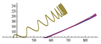
Figure 4. Time plots in phase space. We observe that solutions for different initial conditions, (u(0), v(0)) ∈ {(1, 1), (10, 1), (1, 10)}, converge to different periodic orbits. The vertical and horizontal lines do not correspond to the coordinate axis. They were translated onto the point (400, 120) in order to have a clear view of the region in the first quadrant where periodic orbits appear.
Example 3.4. We consider the following system:
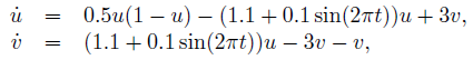
where condition (9) is true. Theorem 2.2 implies the existence of at least one periodic orbit. Here condition (18) does hold therefore the periodic orbit is unique. Numerical evidence supports this claim (see Fig, 5).

Figure 5. Time plots in phase space. We observe that solutions for different initial conditions, (u(0), v(0)) ∈ {(0.01, 0.1), (2, 0.1), (0.2, 1)}, converge to a unique periodic orbit. The vertical and hori[1]zontal lines do not correspond to the coordinate axis. They were translated onto the point (0.42, 0.1) in order to have a clear view of the region in the first quadrant where the periodic orbit appears.

