


 English (pdf)
 Article in xml format
 Article references
 Send this article by e-mail
 Cited by SciELO
  Cited by Google
  Similars in
SciELO
Similars in
SciELO  Similars in Google
 Permalink
1. Introducción
Normally, the methods used for interference tests interpretation are type-curve matching and the conventional straight-line method. In the study by [11] on water flow in aquifers and its influence on water-producing wells, he took the first steps in developing a graphical analysis method that intermediate the field data and the theoretical data for radial regime, which is known as type-curve matching method. Later [2,12,15,18], among others, improved this form of analysis for interference tests by involving either conventional analysis or the pressure derivative function. Type-curve matching is not only tedious but highly inaccurate with a slight data point reading variation.
The first application of the pressure derivative in interference tests was done by [18]. This method did not have much impact at first because it made use of the arithmetic derivative and secondly the noise introduced to the pressure data by external sources increased with the derivative and before the 90s there was not many studies with the estimate of the pressure derivative function. A subsequent analysis was performed by [5], taking as reference the work done by [18] for two-rate testing.
[13] presented the analytical models for radial, linear and spherical flow regimes and used type-curve matching and regression analysis for the interpretation of interference tests. In addition to presenting the analytical interference solution for radial flow regime, [13] also presented the solutions for linear and spherical flow regimes. The first one occurs in elongated deposits caused by channeling or faulting and the second one in very thick formations. [17] followed the philosophy of the TDS Technique, [19], for interference testing using the intersection between pressure and pressure derivative. Later, these recently mentioned works were applied by [7] to determine heterogeneities from interference testing. TDS Technique has many applications, just to name a few of them, [6] and [8] extended this methodology for interpreting pressure tests in elongated systems, and [14] developed the TDS for heavy oil obeying power-law behavior. Much more applications of the TDS Technique were compiled by [9].
Formulating a more practical interpretation methodology for interpretation of interference tests under linear and spherical conditions is the purpose of this paper. For this, the starting points are the linear and spherical solutions presented by [13] so the behavior of pressure and the pressure derivative curves are generated, and, from observations at characteristic points analytical expressions are developed to allow interpreting interference tests in a simple, practical and accurate way. Additionally, based on the work of [3,10], the presence of either pseudosteady-state or steady-state periods was used to develop expressions for the determination of the well drainage area when the duration of the test allows it. The expressions developed were verified satisfactorily with their application to synthetic tests.
2. Mathematical model
For the development of the TDS Technique, [19], in interference tests where either linear or spherical conditions are presented, it is necessary to understand the pressure and pressure derivative behavior in each system with the purpose of finding special features or straight lines which allow obtaining mathematical expressions for reservoir characterization.
2.1. Lineal flow regime model
[16] presented the solution for the pressure distribution in linear systems. This solution was considered for the case of a well producing a constant flow and infinite system. In addition, for an interference test, it was assumed that only half of the active well flow rate is perceived in the observer well. The pressure drop for the described condition is:

And the pressure derivative is given by:

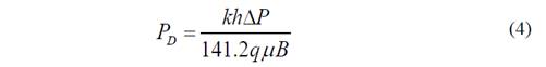
The dimensionless parameters are given as:


Eqs. (1) and (2) allowed generating several pressure and pressure curves as given in Fig. 1 using data from Table 1. As either the reservoir width, b, or the distance between the wells, L, or the reservoir thickness, h, varies so do the pressure and pressure derivative curves; therefore, a unique behavior was obtained after multiplying both dimensionless pressure and pressure derivative and dimensionless time values by certain parameters as shown in Fig. 2. Notice in Eq. (3) that the squared wellbore radius can be changed by drainage area obtained the dimensionless time based on area, tDA .

Source: The authors
Figure 1 Dimensionless pressure and pressure derivative behavior for interference tests under linear flow conditions


Source: The authors
Figure 2 Unified pressure derivative behavior interference tests under linear flow conditions
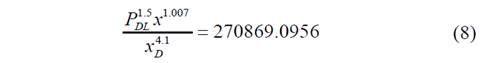
From the unified behavior observed in Fig. 2, a unique intersection point with coordinates 270869.0956, 0.1006 is found:

After replacing the dimensionless time and the definition of dimensionless length, xD =x/L, in Eq. (6), an expression to find porosity was obtained:

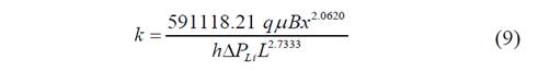
The abscise value was:
From which permeability is solved for once Eq. (4) and xD , are replaced in the above expression:
Since the pressure and pressure derivative values are the same, Eq. (9) can also use the pressure derivative value, instead.
The governing equation for the unique linear flow regime was obtained by regression analysis to be:
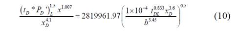
Replacing the dimensionless parameters in Eq. (10) is possible to obtain an expression to find permeability using an arbitrary point during linear flow regime:

Because of the noise introduced to the pressure readings from external sources, it is recommended to read the pressure derivative value during linear flow at a time, t = 1 hr, to obtain a more representative reading value, then, Equation (11) becomes:

The dimensionless pressure governing was found by integration of Eq. (10); therefore:

Dividing Eq. (13) by Eq. (10), and solving for the linear skin factor and replacing the dimensionless quantities, it yields:

2.2. Spherical flow regime model
The governing pressure drop equation for a well producing a constant flow was given by [4] when spherical flow is developed in a reservoir is given by:

Its pressure derivative is then:

As for the former case, pressure and pressure derivative curves were generated, for this case with data from Table 2, considering the variation of wellbore radius, rw , reservoir thickness, h, and distance between wells, r. Such curves are reported in Fig. 3.


Source: The authors
Figure 3 Dimensionless pressure and pressure derivative behavior for interference tests under spherical flow conditions
It was also necessary to unify the pressure derivative curves to obtain a universal behavior. It was performed by multiplying both dimensionless pressure, pressure derivative and time for certain factors as shown in Fig. 4.

Source: The authors
Figure 4 Unified pressure derivative behavior interference tests under spherical flow conditions
From the unified behavior observed in Fig. 4 a unique intersection point with coordinates 0.029163, 0.17513 is found. Therefore,

From which porosity is obtained once the dimensionless quantities are used:

and;

After replacing Eq. (4), the definition of dimensionless radius and solving for the formation permeability, it yields.

Since the pressure and pressure derivative values are the same, Eq. (20) can use the pressure derivative value, instead.
The governing universal equation for spherical flow was obtained by linear regression to be:

Replacing the dimensionless parameters in Eq. (21), it is possible to obtain an expression to find permeability using an arbitrary point during linear flow regime:

As for the linear case, because of the noise, it is recommended to apply Eq. (22) at the time of 1 hr.
The dimensionless pressure governing equation was obtained by integration of Eq. (25), to be:

Dividing Eq. (23) by Eq. (21), replacing the dimensionless quantities and solving for the spherical skin factor will result:

2.3. Late time behavior
The basis for interference in bounded systems were given by [3]. The application of the pressure derivative for limited reservoirs was presented by [10]. This means that it is feasible to develop either pseudosteady-state or steady-state periods during an interference test. As observed in Fig. 5, once spherical flow regime vanishes pseudosteady-state period obeys the following governing pressure derivative equation:

Replacing the dimensionless quantities and solving for the drainage area, it results:

As shown in Fig. 6 the pressure derivative governing equation is given by:

As for the spherical flow case, after replacing the dimensionless time based on area, the resulting area equation was:


Source: The authors
Figure 5 Dimensionless pressure behavior versus dimensionless time based on area for spherical flow interference in closed systems

Source: The authors
Figure 6 Dimensionless pressure behavior versus dimensionless time based on area for linear flow interference in closed systems
On the other hand, for constant-pressure bounded systems, Figs. 7 and 8, the late-time governing pressure derivative equations for linear and spherical flow regimes, respectively are given by:

Replacing the dimensionless quantities and solving for the drainage area results in:

As shown in Fig. 8 the pressure derivative governing equation is given by:

Replacing the dimensionless quantities and solving for the drainage area, it results:


Source: The authors
Figure 7 Dimensionless pressure behavior versus dimensionless time based on area for spherical flow interference in constant-pressure systems

Source: The authors
Figure 8 Dimensionless pressure behavior versus dimensionless time based on area for linear flow interference in constant-pressure systems
Because of the noise, it is recommended to apply Eqs. (28), (30) and (32) at time of 1 hr.
The spherical system can be readily converted to hemispherical system. As seen in Eq. (15), the constant (sp has the value of 70.6. For hemispherical flow conditions this constant is multiplied by two, taking the value of 141.2, so do the constants in the related equations. Apart from this, appendix A presents the gas flow equations for linear and spherical flow conditions.
3. Examples
Two synthetic examples were generated to validate the porosity and permeability equations and two other tests were synthetically created two verify the equations of area. Table 3 contains the input data for the examples.

3.1. Example 1 (Linear)
The simulated data provided in Fig. 9 was generated with data from Table 3, from where the following information was read:


Source: The authors
Figure 9 Log-log of pressure and pressure derivative versus time for example 1 (linear case)
Then, permeability was estimated with Eqs. (9) and (11) and porosity with Eq. (7). Results are reported in Table 4.

3.2. Example 2 (spherical)
Fig. 10 presents the pressure and pressure derivative data for a synthetic test under spherical flow interference conditions which used input data from Table 3. The following information was read from such plot:
Source: The authors
Figure 10 Log-log of pressure and pressure derivative versus time for example 2 (spherical case)

Permeability was estimated using Eqs. (20) and (22). Porosity was found with Eq. (18). Results are also reported in Table 4.
3.3. Example 3 (spherical case)
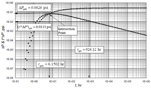
A long pressure test was also simulated with input data from Table 3. The pressure and pressure derivative for this example is reported in Fig. 11 from where the following characteristic point was read:

Drainage area was estimated with Eq. (30) -reading at t = 1 hr- and reported in Table 4.


4. Conclusions
The intersection point, a characteristic one-half slope (for linear flow) and negative one-half slope (for spherical) flow, a late time unit-slope line (pseudosteady state) and a late time negative unit-slope line (steady state) are identified and set as characteristic features on the pressure and pressure derivative versus time log-log plot which allow developing expressions for reservoir characterization.
TDS Technique is applied to interference testing under linear and spherical flow regime conditions. A unique point of intersection - found for each case - is used to find expressions to find reservoir permeability and porosity. Also, the permeability value is verified by another expression that uses an arbitrary point read on each flow regime (linear or spherical). There are also developed equations to estimate the drainage area in both dealt flow regimes for close or constant-pressure boundary systems. The Equations are successfully verified on synthetic cases.
Nomenclature

Suffixes

Greek


