


 English (pdf)
 Article in xml format
 Article references
 Send this article by e-mail
 Cited by SciELO
  Cited by Google
  Similars in
SciELO
Similars in
SciELO  Similars in Google
 Permalink
1. Introduction
The human visual system (HVS) can process large amounts of visual information instantly and is able to locate objects of interest and distinguish them from complex background scenes. Research shows that the HVS pays more attention to infrequent features and suppresses repetitive ones [1-2]. Visual saliency plays an important role in the process in which HSV identifies scenes and detects objects. It is also concerned with the way the biological system perceives the environment. For example, every time we look at a specific place, we pay more attention to particular regions which are distinct from the surrounding area.
Visual saliency is an active research field in areas such as psychology [2], neuroscience [3], computer vision [4-5] and computer graphics [6-7]. There are many computational methods for simulating the HVS and visual saliency, but it nonetheless remains an unexplored field because of the difficulty of designing algorithms to simulate this process [6]. As for computer graphics, while the concept of visual saliency has been widely explored for mesh saliency [6], [8-18], few studies have explored visual saliency in point clouds [19-22]. Visual saliency is an important topic for 3D surface study and has important applications in 3D geometry processing such as resizing [1], simplification [23-24], smoothing [25], segmentation [26], shape matching and retrieval [27-28], 3D printing [29], and so forth.
Due to the development of 3D data scanning technology, current scanners generate thousands of points for every scanned object. Therefore, for rendering, point clouds have become an alternative to triangular meshes. A common way to process a point cloud is to reconstruct the surface using methods such as triangular mesh, NURBS representation and Radial Basis Functions. However, due to a large number of points, different sampling densities and the inherent noise produced by the scanning process, reconstruction is an expensive and challenging computational task. For these reasons, it is necessary to develop geometry processing algorithms that operate directly on the point sets. Applying existing saliency detection techniques to point clouds is not a trivial task. This is due to the absence of topological information, which is not a problem for mesh-based methods. The method we propose here is inspired by Li et al. [30] and we made it fit for general use supported by the Minimum Description Length (MDL) principle. In this way, MDL is used as a criterion to distinguish regions in the point clouds.
1.1. Contribution
The main contributions of this paper are: (1) a method for saliency detection without topological information using only the raw point sets, (2) the use of the MDL principle for defining saliency measurements, extended to sparse coding representation to obtain saliency maps of point clouds.
Experimental results show that the proposed algorithm performs favorably in the capture of the geometry of the point clouds without using any topological information and achieves an acceptable performance when compared to previous approaches.
1.2. Organization
This paper is organized as follows. A review of related work on saliency detection is provided in Section 2. The theoretical basis for Sparse Coding and MDL for the proposed Sparse Coding Saliency method is presented in Section 3. Section 4 lays out the results and discussion. Finally, we present the conclusions and future studies in Section 5.
2. Related work
Visual saliency detection has its origin in the area of computer vision, specifically in 2D images. Inspired by this research, visual saliency detection has been applied successfully to 3D meshes and point clouds. In recent years, much research has tried to develop methods for visual saliency on 3D surfaces [10-12,17,19-21,32].
Early advances in the field of Mesh Saliency used 2D projections for 3D applications. While such works often ignored (or were unable to exploit) the importance of depth in human perception, they set a basis for further research by highlighting the importance of human perception in image analysis [18]. Some of the first researchers to exploit saliency for 3D mesh processing were Lee et al. [32]. The authors introduced the concept of mesh saliency and computed it using a Gaussian-weighted center-surround mechanism. Results were then exploited for the implementation of mesh simplification and best point-of-view selection algorithms. Wu et al. [13] presented an approach based on the principles of local contrast and global rarity. This method has applications for mesh smoothing, simplification and sampling. Leifman et al. [33] propose a method for detecting a region of interest on surfaces where they capture the distinctness of the vertex descriptor, characterizing the local geometry around it. The method is applied to viewpoint selection and shape similarity. Tao et al. [11] put forward a mesh saliency detection approach which reached state-of-the-art performance even when handling noisy models. Firstly, the manifold ranking was employed in a descriptor space to imitate human attention, and then descriptor vectors were built for each over-segmented patch on the mesh, using Zernike coefficients and center-surround operators. Afterward, background patches were selected as queries to transfer saliency, helping the method to handle noise better. An approach for mesh saliency detection based on a Markov Chain is proposed by Liu [10]; the input mesh was partitioned into segments using Neuts algorithms and then over-segmented into patches using Zernike coefficients. Instead of employing center-surround operators, background patches were selected by determining feature variance to separate the insignificant regions. Limper et al. [8] applied the concept of Shannon entropy, which is defined as the expected information value within a message, for 3D mesh processing. In this case, the curvature is established to be the primary source of information in the mesh. Song et al. [18] argued for the benefits of using not only local but also global criteria for mesh saliency detection. Their method consisted of computing local saliency features while considering the later computation of global saliency using a statistic Laplacian-based algorithm which captures salient features at multiple scales.
Recently, point saliency detection-based methods have been introduced. Shtrom et al. [21] propose a multi-level approach to find distinct points, basing their approach on the context-aware method for image processing. Tasse et al. [20] propose a cluster-based approach; the method discomposed the point cloud into the small clusters using an adaptive fuzzy clustering algorithm and is applied in the detection of key-points.
Finally, Guo et al. [19] propose a saliency detection method based on a covariance descriptor to capture the local geometry information, using a sigma set descriptor to transform the covariance descriptor from a Riemannian space to a Euclidian space to facilitate the application of Principal Component Analysis for the inner structure analysis to classify whether a point is salient or not.
3. Proposed method
The saliency detection framework based on sparse coding is shown in Fig.1. The input point cloud is represented in sparse form and the saliency is estimated by a center-surround hypothesis [34-35], which states that a region is salient if it is distinct from its surrounding regions. Taking a point cloud as input, we estimate a neighborhood with radius r for each point in the cloud, then select some of its boundary points. We estimate a neighborhood with radius r around each selected point. Overlapping is allowed between neighborhoods in order to capture the structure of the cloud. Then, for each point in the neighborhood, we compute a set of basic features to build a descriptor vector and finally, we estimate the mean of the feature vectors to build only one descriptor vector per neighborhood. Similarly, we do the same with the neighborhoods surrounding the central one. Afterward, we construct a dictionary D, using the feature vectors from the surrounding neighborhoods, and then a sparse coding is carried out using the feature vector of the central neighborhood and by searching for a sparse representation for it with the basis in the dictionary D. Finally, we compute the neighborhood saliency using the MDL principle based on the sparse representation measure of vector x, and the residual of the sparse reconstruction measure. The final saliency map is computed using a fusion of both measures.

Source: The Authors.
Figure 1. . Processing pipeline of our sparse coding-based saliency detection method.
3.1. Sparse coding
The purpose of sparse coding is to approximate a feature input vector as the linear combination of basis vectors, called atoms, which are selected from a dictionary which has been created from the data. In other words, sparse coding provides a low-dimensional approximation of a given signal in a given set of a basis [36].
Formally, let
 be a signal of dimension
 , the sparse coding aims to find a dictionary
 such that
 can be approximated by a linear combination of the atoms
 this is
 (if the dictionary is overcomplete then
 where most of the coefficients
 are zeros or close to zero [37]. We propose that the sparse coding problem can typically be formulated as an optimization problem, as in (1):

In this formulation, the dictionary D is given and L controls the sparsity of x in D. The term
 measures the dispersion of the decomposition and can be understood as the number of non-zero coefficients in
 , or, sparse coefficients, in order to approximate the signal
 in as sparse a way as possible. Or, alternatively, it can be formulated as (2):

This is an optimization problem where the norm
 is changed by the norm
 , where
 is the regularization parameter). The solution to equation (1) with the norm
 is an NP-hard problem; fortunately, under certain conditions, it is possible to relax the problem using the norm
 and find an approximated solution using equation (2) with the norm
 .
.
3.2. Minimum description length
The Minimum Description Length (MDL) principle [4][31][38] states that, given a model class
 of candidate models, its parameter M, and its data sample x, the MDL will provide a generic solution to the model selection that minimally represents the data x. Formally, given a set of candidate models
 , and a data vector
 , MDL searches for the best model
 , that can be used to describe x in its entirety with the shortest length.

 is a coding assignment function which gives the codelength required to describe
  uniquely.
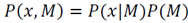
In [39], a method based on information theory was introduced for image saliency detection. This method measures the saliency concerning the likelihood of a patch given the patches that surround it. The method measures the self-information using the negative log-likelihood. Defining
 as an image and
 as the probability of occurrence of the patch
  , given its surrounding neighborhood patches, the saliency measure of the patch is defined
 that is, the self-information characterizes the raw likelihood of the n-dimensional vector values given by
 .
.
Based on [4,31,38], we use the MDL principle to propose a method for salience detection in point clouds based on sparse coding. The coding assignment function can be defined in terms of probability assignment
 based on the Ideal Shannon Codelength Assignment [28], that is,
 . Using Bayes theorem, we can establish
 as
as
 and then by applying maximum a posteriori (MAP), the penalized likelihood form of the coding model is formulated thus:

Where
 is the term that describes how well the model adjusts the data
and
is the term that describes how well the model adjusts the data
and
 describes the model complexity, model cost or prior term.
Once
 is estimated, the terms in equation (4) can be interpreted as follows:
 is the description length or codelength of the model; and
 is the description length or Codelength of the data encoded using the model.
3.3. Relating the MDL principle to sparse coding
The standard Gaussian is assumed to be coding assignment function
 , and assuming that
 can be represented in a sparse way given a basis dictionary
 and a sparse vector
 , the probability distribution of the reconstruction error follows a Gaussian distribution
 with known variance
 . The term
 in (4) becomes
 , and the term
 in (4), assuming sparsity constraint, becomes

 . The aforementioned calculations adhere to the sparse coding model described in Section 3.3.
The sparsity condition and the sparse reconstruction error conform to the MDL principle if we set the estimation parameter
 and evaluate it with the prior term and with the likelihood term
 and so
 and
and
 are obtained respectively. We conclude that the sparsity of the vector
  is the codelength of the model and the residual of the sparse reconstruction error is the codelength of the data given the model.
The MDL principle selects the best model that produces the shortest description of the data. The more regularity that is presented in the data, the shorter the description the model will produce. If a neighborhood is equal or slightly different with respect to its surroundings in terms of information, it means these signals (neighborhoods) are redundant and can be represented sparsely with a suitable basis dictionary, meaning that its description length (the sparsity of vector
 i.e.,
i.e.,
 will be short and we can conclude that this neighborhood is not salient; on the other hand, if the neighborhood is very different from its surroundings, its description length will be longer. In other words, it cannot be represented sparsely by the basis dictionary and we can conclude that the neighborhood is salient.
If the sparse reconstruction error (i.e.,
produces a high residual, it means that its description length will be longer and this implies that the neighborhood is dissimilar from its surroundings and therefore more salient. On the other hand, if the sparse reconstruction error produces a low residual, its description length will be short and this implies that the neighborhood is similar with respect to its surroundings and, consequently, less salient. Based on these saliency measurements, our point cloud saliency detection method is described below.
3.4. Sparse coding saliency detection
Unlike some saliency detection methods for point clouds compiled in the literature review, our method does not estimate saliency using individual points directly, rather, a neighborhood is used to determine its saliency.
3.4.1. Feature vector
Given the point set
 , a neighborhood i
 is estimated for every point
 with radius ,
 is the number of neighbor points
 inside a sphere with radius
 , and center
 See Fig.1. In order to establish whether a neighborhood is different, first it is important to characterize it with a descriptor, of which there are several which describe low level features for each
, for example, normal, curvatures, shape index, etc. In this method the normal and Gaussian curvatures are selected; these features are rotationally invariant. A third feature ,
See Fig.1. In order to establish whether a neighborhood is different, first it is important to characterize it with a descriptor, of which there are several which describe low level features for each
, for example, normal, curvatures, shape index, etc. In this method the normal and Gaussian curvatures are selected; these features are rotationally invariant. A third feature ,
 , is also selected. With the features defined, a five dimensional feature vector
 is formed for every point
 of
of
 , i.e.,

 where
where
 are the three components of the normal vector
 ;
;
 is the Gaussian curvature and
 is the fifth component coordinate of
 , which will be defined below. It is necessary to have a single descriptor vector for each neighborhood, so the mean of the characteristic vectors belonging to the neighborhood are estimated as follows:

Where
 is the cardinality of

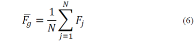
 is a global measure, which establishes the difference between the feature vector of each neighborhood
 and the global mean
 (6) of all the feature vectors of the point cloud, that is:

3.4.2. Surrounding neighborhoods
Once the neighborhood descriptor is established, the next step is to find the surrounding neighborhoods to each  To find these neighborhoods, first, the 3x3 covariance matrix (8) of
 is computed as:

Where
 is the mean of
 and
and

After the covariance matrix
 has been estimated, we will use its two largest eigen-values with its corresponding eigen-vectors that follow the
 and
and
 axes, which expand the tangent plane
 to
to
 . at the point
 . Next, the points within
 are projected onto the 2D plane
 as shown in Fig. 2(a). Before projecting the points within
 we establish the area of the surrounding neighborhoods as the n-ring, as can be seen in Fig. 2(b), that is, the 1-ring corresponds to radius
 , the 2-ring corresponds to
 and so on. In these experiments we used the 1-ring. Then, we proceed to trace a set of radii, separated by an
 angle, from the center of the projected neighborhood in Fig. 2(b); the length of radii is n-ring. In each of the radii, we mark points (green dots) depending on if we have used the 1-ring, 2-ring or n-ring, as shown Fig. 2(b) Then, we find the nearest point to each marked point within the projected neighborhood and find its corresponding point within the 3D neighborhood; then we estimate a neighborhood for each of the 3D points with radiusr, as seen in Fig. 2(c). Finally, a feature vector is estimated for each surrounding neighborhood, in the same way as in the previous section.
3.4.3. Dictionary construction and sparse coding model
It can be observed that the surrounding feature vectors
 are a natural over complete basis dictionary

 and the central feature vector
 acts as the sparse linear combination of these basis or atoms, i.e.
 , Now we can write the sparse model as so:
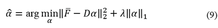
Equation (9) is a linear regression problem optimization for estimating
 , known as Lasso. The LARS algorithm gives the solution and the SPAMS library is used to carry out the sparse coding solution.
3.4.4. Saliency detection
Previously, in Section 3.4.1,
 was mentioned as being the fifth component of the feature vectors
 , and it was estimated using (7). This component was added because often, a local neighborhood has similar surroundings but the local and surroundings are globally distinct over the entire point cloud. Using only normal vectors and Gaussian curvature can produce areas in the cloud which have saliency but the center of these areas can be empty. Adding
 solves this difficulty.
When a sparse solution to (9) is achieved, the codelength for the neighborhoods is established as was laid out in Section 3.3. Our model is based on the MDL principle, therefore, the saliency of each neighborhood
 is proportional to
 . We replaced the L2- norm with the L1-norm in the residual error, because it is more discriminative and robust to outliers. Next, following the instructions in Borji and Itti [40], we rewrote the equations
 and
and

 both saliency measurements are then normalized and combined (10).

Where
 is the saliency produced by the sparse reconstruction error,
 is the saliency produced by the sparse coefficient and
 is the combination of both saliency measurements;
 normalizes the saliency measurements for a better fusion. The symbol
 in (10), is an integration scheme
 [40], see Fig. 3.

Source: The Authors.
Figure 2 Surrounding neighborhoods selection. (a) Projecting the 3D points to 2D, (b) mark points and n-ring area, (c) selecting surrounding neighborhoods.
Source: The Authors.
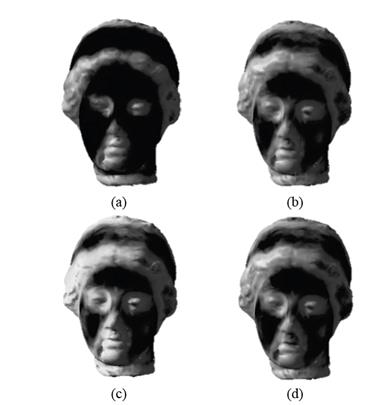
Figure 3 Saliency maps generated by different operator functions, using equation (11). (a) Using * operator, (b) Using + operator, (c) Using min operator and (d) Using max operator.
The best results in all experiments were produced using the * operator. Since overlapping is allowed between neighborhoods, the total saliency map is obtained by accumulating the saliency by neighborhood. Our method differs from that proposed in [30], since it only uses the dispersion vector (i.e.,
 )as a measure of saliency, while our method also takes into account the reconstruction error or residual (i.e.,
 )as an additional measure of saliency; finally when these measurements are combined, we obtain a better saliency map. Our method can be seen as a generalization of the framework presented in Li et al. [30], improving the final result of the saliency map. This can be observed in Fig. 4. This is a result of the residuals performing as a weighting factor with respect to the measure of rarity given by the dispersion vector.


4. Results and discussion
In this section, we evaluate the proposed method on a set of objects and compare it against 3D model saliency detection approaches outline in the literature review, taking into account methods based on point clouds and meshes. The object shapes were obtained from the Watertight Models of SHREC 2007 and the Stanford 3D Scanning repository. Our method is compared to three-point cloud-based methods from the literature review: Tasse et al. [20], Shtrom et al. [21] and Guo et al. [19], as well as six mesh-based methods from the literature review: Lee et al. [32], Wu et al. [13], Leifman et al. [33], Tao et al. [11], Song et al. [18] and Liu et al. [10]. It is also compared against the pseudo-ground truth [41].
All the experiments were run on a PC with an Intel Core i7-2670QM CPU@2.20 GHz and 8GB RAM. As an example, for the model of a girl in Fig. 8, with 15.5 K vertices, the saliency computation cost of our method was 81.7s, being slower than Tasse [20] and Guo [19] but it has some optimizations and if a language like C++ is used, performance will improve.

Source: The Authors.
Figure 5 Saliency map produced by our method with different values of λ. From left to right: λ = 0.1, 0.2, 0.4, 0.6, 0.8, 0.9.

Figure 6 Point-based methods saliency comparison. (a) Shtrom et al. [23]. (b) Tasse et al. [3]. (c) Guo et al. [24], and (d) our proposal.

Source
Figure 7 Mesh-based methods comparison. (a) Lee et al. [21]. (b) Wu et al. [10]. (c) Leifman et al. [22], Tao et al. [8] (d), and (e) our proposal.

4.1. Parameter selection
The only parameter in our method is
 ; this is the regularization parameter. It produces smoother results as value increases in the range (0, 1); its visual effect is appreciated in Fig. 5. Experimentally we found that, on average, a value of lambda of near to 0.9 generates the best qualitative as well as quantitative results, therefore in all our experiments, we fix lambda at
 .
.
The size of the neighborhood is calculated according to the local characteristics of points like density and curvature, and its size is increased or decreased. To achieve this, a method -such as that proposed in [42]- is used to estimate the size of the neighborhood, taking into account the local characteristics named.
4.2. Qualitative evaluation
Our method is compared with methods from the literature review, both mesh-based and point cloud-based. In Fig. 6, we compare the point-based methods, including Shtrom et al. [21], Tasse et al. [20] and Guo et al. [19]. The method in Shtrom et al. can obtain a reasonable saliency result and highlights a relevant saliency region on the Max Planck model, but there are also extensive areas with noise around the principal saliency features. In the method proposed by Tasse et al., less noise is perceived, but there are large regions around the features with greater saliency. In the result of the Guo et al. method we observe a clean saliency map concentrated on the most representative saliency features, however, our result, in addition to achieving the same, highlights areas such as eyes, the lower part of the nose, ears and lips with greater saliency. Regarding the dragon model, there was a similar result as with the Max Planck model. The proposed method produces a clean saliency map compared to Shtrom et al. and Tasse et al. The saliency map produced by Guo et al. is very similar to ours, which only highlights some of the finer details such as eyes and ridges.
We also compare our results with mesh-based methods, shown in Fig. 7, with those of Lee et al. [32], Wu et al.[13], Leifman et al. [33], and Tao et al. [11]. It can be observed that the local changes in the curvature had less influence when using the proposed method, as seen in Lee et al. [32].
In the bunny and dragon models, the saliency map is not correct due to variation of the level of saliency in different areas, the dragon, for example, has lost some fine details like crests and ridges.
The method of Wu et al. produces a better saliency map than that of Lee et al., but some salient areas are missing as in the case of the dragon. The method proposed by Leifman et al. produces a reliable saliency map for the dragon model, in the case of bunny, the feet are missing in the final saliency map. For the Tao et al. method, it can be seen that in the dragon model, some areas are shown to be salient where they are not. In the visual comparisons, it should be pointed out that our method generally achieves better results than the other four methods.
Fig. 8 compares our results with [10,11,18], and shows that the way in which our method detects saliency is more coherent, as it detects small salient regions, such as the ears and the little tie, and the facial regions like the eyes and mouth of the bust of the girl. Furthermore, the hair (bun and braids) show up better with the pseudo-ground truth [41], in comparison to the other four methods. We observe, in reference to the bird model, how our method detects the saliency points in the wings, tail, beak and finally the light area of saliency between the wings compared to the pseudo-ground truth bird model.

Source: [11].
Figure 9 . Saliency results on Gargoyle model. Our method (bottom row), and Tao et al. [11] (first row). The first two columns are front and back view of saliency results from Gargoyle model. The second two columns are the same view results but with 30% random noise relative to the average of the nearest distance of each point.
Fig.9 shows the results when the input is a noisy point cloud, we can observe that our method is more robust against noise in comparison to mesh-based methods [11]. We added 30% (relative to the average of the nearest distance of each point) random noise to disturb the points’ coordinates, and observe that the method proposed by Tao et al. failed to detect some details of the wings in the gargoyle like the little rings between the veins from the front view and the loss of some details in the veins from the back view. We can observe that our method is more consistent in detecting salient features in the gargoyle model, both in the clean and noisy model in comparison to Tao et al. [11]. The strength of our method lies in the fact that since the saliency of point clouds is a feature of a sparse nature, modeling based on sparse models is usually a good alternative to adequately represent these characteristics. When it is combined with the MDL principle, this method is the simplest and best choice guarantee among all the possible solutions.
4.3. Quantitative evaluation
We carried out a quantitative evaluation on the 400 watertight models of SHREC 2007, using the distribution of schelling points provided by Chen et al. [41] as the ground truth. To evaluate the performance, we used the metrics proposed by Tasse et al. [43]; they propose three metrics that adapt 2D image saliency metrics to 3D saliency, these metrics are: Area Under the ROC curve (AUC), Normalized Scanpath Saliency (NSS) and Linear Correlation Coefficient (LCC). In the AUC metric the ideal saliency model has a score of 1.0, AUC disregards regions with no saliency, and focuses on the ordering of saliency values. The NSS metric measures the saliency values selecting the users as fixation points. The LCC metric has values of between -1 and 1, with values closer to 0 implying weak correlation. This metric compares the saliency map under consideration with the ground-truth saliency map (Schelling distributions). For comparison, we selected three methods from the literature review, two based on point clouds and one based on meshes, these methods are: the clustering method (CS) [20], the point-wise method (PW) [19] and the spectral analysis method (SS) [12]. Also, as a reference score, we incorporated the human performance score (HS), provided by Tasse et al. [43].
Table 1 shows the AUC score values of the selected methods; our method competes with the CS and PW methods, as the final average shows. The SS method performs poorly compared to our method and the CS and PW methods. The same is true regarding the HS method which outperforms the SS method. Table 1 shows that for the classes glasses, ant, octopus, bird and bearing, our method obtained the best results, while for the classes hand, fish, spring, mechanic, airplane and vase, our method equals the PW and CS methods. The above shows that the proposed method achieves the same as the most up-to-date methods of the literature review and, in some cases, even improves on them.

Fig. 10 shows NSS and LCC metrics, and also confirms that the performance of our method is similar to CS and PW, and outperforms SS, but HS outperforms all methods presented.

5. Conclusions and future work
This paper presents a novel and simple method for point cloud saliency detection via sparse coding. Based on the MDL principle, the proposed method uses a sparse coding representation to find the minimum codelength to establish when a neighborhood is salient or not with respect to its surrounding neighborhoods. It is robust against noise since it takes the mean of the feature vectors of the neighborhood as a unique feature vector.
Our approach produces feasible and even faithful results on a variety of models, giving convincing results. We have compared our results to the most recent approaches found in the literature review and we found that the proposed method competes with and in several cases significantly outperforms these approaches, using the pseudo-ground truth provided by Chen et al. [41] as a reference. For future studies, we plan to investigate how the incorporation of high-level information in the form of semantic cues into the point cloud saliency detection allows us to identify salience globally on the point cloud.

