


 English (pdf)
 Article in xml format
 Article references
 Send this article by e-mail
 Cited by SciELO
  Cited by Google
  Similars in
SciELO
Similars in
SciELO  Similars in Google
 Permalink
1. Introduction
The educational transformation based on competencies and learning outcomes has caused the way of teaching and evaluating to change. The current teaching times have decreased concerning the increase of study time by the student, requiring the use of educative technological tools that support the training process in the classroom and the student’s autonomous learning, especially in these post-pandemic times and the technological changes that impose new ways of teaching. These new dynamics lead to the urgent need to develop teaching-learning tools that support the student’s autonomous work and the methods of teaching mediated by technological means. On the other hand, the accompaniment of engineering teaching with computational tools introduces the experimental character necessary when developing computational laboratory practices.
Pedagogical strategies mediated by technological learning tools strengthen education and consolidate quality student learning outcomes. Mainly, teaching the mechanics of deformable solids can be complex due to the difficulty in understanding the phenomena that govern the problems, mathematical theories, and mechanical performance characteristics. In the new learning contexts, solving plane stress problems and deformations involving strain energy and drawing Mohr’s circle by doing operations by hand and drawings on sheets of graph paper is a past task. Hence the importance of supporting the teaching of these topics with computer calculation tools.
Educational applications for teaching the mechanics of deformable solids to engineering students are scarce. It is not common to find non-commercial educational software that assists in the step-by-step calculation of these problems. In addition, some computer applications that exist to help study some topics in mechanics of materials and solving problems are not readily available and, therefore, cannot be used by students. Other recent applications are only in English [1,2] and are not user-friendly. So, the developed application is justified as it calculates efficiently and in an understandable way for the student all the study variables of the plane stress problem. In other words, it fully develops the plane stress problem, the associated deformations, and the strain energy and plots Mohr’s circle of stresses. Furthermore, the educational application is available in English and Spanish, has a user’s manual, and uses a free compiler that links with the free Computer Algebra System MAXIMA available in Windows and Linux. For this reason, the EsfPlano2D program is a multiplatform educational application, free to use and easy to access.
Other tools focused on teaching and learning the Mohr circle have been developed in the past; however, there was no access to them. For example, in [3], an educational program for computer-assisted education on Mohr’s circle and its practical use is presented. The educational tool was implemented as part of a finite element analysis program. In [4], the results of academic applications for mechanics courses that can be used for engineering analysis and practical design of structural and machine elements are presented. In [5], it is shown how a circular Mohr diagram can represent a triaxial state of stress and strain if appropriate scale changes are made. In [6], the development of an instrument for an oscilloscope that provides information about the Mohr circle is presented. More recently, [7] proposed to plot Mohr’s circle and principal stresses using Mathcad software. In [8], a learning tool was presented that shows the stress state and its corresponding Mohr’s circle at a point of a structure. Similar works with educational approaches to visualize Mohr’s circle for plane stresses are also presented in [9-12]. Finally, in [13-17], several investigations are presented using Mohr’s circle to find out, e.g., the failure state of a material, stress intensity factors, and large deformations.
This paper is divided into four sections. First, a theoretical framework of the plane stress issue is presented. Then, the methodology is developed. After, the results obtained with the tool are presented, and finally, the conclusions and recommendations are drawn.
2. Theoretical framework
The stress conditions present in structural members subjected to axial, torsional, and bending effects represent a plane state of stress. In the engineering design of structural members subjected to some of these effects, the normal and shear stresses present in the cross-sections of the members can be obtained from formulas. However, the maximum stresses that must be calculated for design purposes occur in inclined planes. Thus, inclined sections along the member may be subjected simultaneously to normal and shear stresses, usually more significant than those acting in the cross-section. Mohr’s circle is a general technique for determining stresses in inclined planes. The procedure requires stress elements to represent the stress state at a given point in a body. The educational application EsfPlano2D uses Mohr’s circle to determine the normal and shear stresses acting on inclined sections of members from the stresses in the cross-sections. In other words, Mohr’s circle determines the stresses acting on the sides of a stressed element rotated to any position, starting from the stresses at the reference position [18].
In Mohr’s circle, when an element is rotated from one position to another, the stresses acting on the faces of the element are different but represent the same stress at the point considered. The situation is analogous to the representation of a vector by its components. The force is defined by its components but without modification of the force itself. However, the state of stress at a point of a body is a more complex quantity than a force, and the transformation relations for stresses are more complex than for vectors.
Only a two-dimensional view of the stressed element is represented to analyze plane stress. For example, normal tensile stress is positive from the face. Likewise, shear stress is positive when acting on a positive face of the element in the positive direction of an axis and negative when acting on a positive face in the negative direction of an axis.
Starting from the stresses in the cross-section, (x, (y, (xy, the stresses acting on the inclined section are calculated, considering another stressed element whose faces are perpendicular and parallel to the inclined section so that, to this new element are associated the x1, y1, z1 axes. The z1-axis coincides with the z-axis, and the x1y1 axes are rotated by an angle ( counterclockwise concerning xy-axes. The normal and shear stresses acting on this rotated element are denoted by (x1, (y1, (x1y1. The transformation equations for plane stress determining the normal and shear stresses on the inclined plane x1 as a function of the angle of rotation ( and the stresses((x, (y, (xy acting on the x and y planes of the cross-section are shown in eqs. (1) to (3).


Equivalent normal stresses act on the planes of maximum and minimum shear stresses equal to (average, as shown in eq. (4).

In the transformation equations for plane stress, the normal stress (x and the shear stress (xy vary with the angle (. For design purposes, the maximum positive and negative values of the stresses are necessary; therefore, the ( values for which( x1 is the maximum or minimum can be found with the cosine function of the double angle, as shown in eq. (5).

The angle 2θp has two values that differ by 180°. For one of these two angles, the normal stress σx1 is the maximum and minimum principal stress for the other. The more considerable principal stress is denoted by σ 1 and the minimum by σ 2 and act in perpendicular planes. The angles at which the shear stresses (x1y1 acting on rotated elements occur are calculated by eq. (6).

The maximum and minimum shear stresses differ only in sign and occur at 45° to the principal planes. Therefore, the shear stresses are zero on the principal planes, and the maximum shear stress is determined according to eq. (7).

The transformation equations for plane stress can be represented by a graph known as Mohr’s circle. This representation makes it possible to distinguish the relationships between normal and shear stresses acting on inclined planes at a point on the stressed element. The transformation equations are arranged to draw Mohr’s circle, and the equation of the circle of coordinates (x1 and (x1y1 and radius R of eq. (8) is found.

Where R is
 . On Mohr’s circle, (x1 is the abscissa axis, and (x1y1 is the ordinate axis. The angle( for the stressed element is positive counterclockwise. Therefore, the angle 2( p on Mohr’s circle is positive counterclockwise.
Now, to calculate the normal deformations produced by the normal stresses, including the Poisson ratio (( ), Hooke’s law for normal stresses is applied, as shown in eqs. (9) to (11).


The unit volume change (e) is determined by the sum of the three normal strains or, as a function of the normal stresses, by eq. (12).

The angular deformation produced by the shear stress is determined by applying Hooke’s shear law given by eq. (13), and the strain energy density is calculated according to eq. (14).


Similarly, the transformation equations for the plane strain determining the normal and angular deformation on the inclined plane x1 as a function of the angle of rotation ( and the strains (x, (y, (xy acting on the xy-planes of the cross-section, can be calculated through eqs. (15) to (17).


Now, the major principal deformation denoted by ε 1 and the minor one denoted by ε 2 acting in perpendicular planes, are calculated with eqs. (18) and (19), and the principal angles( p and( s for the normal and angular deformation are found with eqs. (20) and (21), respectively.


Likewise, the average normal and maximum angular strain is calculated using eqs. (22) and (23).


3. Methodology
The EsfPlano2D is an educational computer program developed in the Fortran language that links to the free Computer Algebra System MAXIMA to plot Mohr’s circle of stresses. The steps shown below must be followed to prepare the program for the calculation of a plane stress problem:
a)Copy the installation files folder named Esfplano2d to the root C: of the computer.
b)Inside the Esfplano2d file folder, find the MAXIMA installation file named maxima-5.46.0-win64.exe and install it. To install the MAXIMA program, run the installer as an administrator with the right mouse click.
c)Install the MAXIMA program in the root C: of the computer and verify that the program is installed in the folder named maxima-5.46.0.
d)Please find in the installation files folder of the educational application Esfplano2d the shortcut of the application executable named EP2d, copy it, and then paste it on the computer’s desktop.
e)Run the educational application Esfplano2d by double-clicking on the shortcut.
f)Antivirus may identify the application as a threat. If this happens, please add it as an exception in Antivirus.
g)The Esfplano2D program is ready to calculate.
The program asks for the name to be assigned to the results file when it is executed by double-clicking on the shortcut (see Fig. 1).
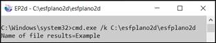
A name, preferably shorter than fifteen characters, should be assigned. Thus, the results file will be created with the name given to the file and the extension *.res. This results file will be located inside the application’s installation folder in root C. Next, the program asks for the input stress values (Sigma x; Sigma y; Sigma xy; Teta (°); Modulus of Elasticity E and the Poisson Ratio). Sigma x is the normal stress (x; Sigma y is the normal stress (y; Sigma xy is the shear stress (xy; Theta is the angle of rotation in degrees ((°) of the xy plane. Additionally, the values of Modulus of Elasticity (E) and Poisson’s ratio (( ) should be entered for the deformation calculations using Hooke’s law, as shown in Fig. 2.
A results screen is displayed when the plane stress problem calculations are finished. Table 1 describes the parameters displayed in the results screen and their meaning.
Table 1 Meaning of output parameters
| Parameter | Meaning | |
|---|---|---|
| sx | = | Normal stress in the x-direction |
| sy | = | Normal stress in the y-direction |
| sxy | = | Shear stress in the xy-plane |
| T | = | The angle of rotation of the x and y-axis (counterclockwise) |
| x1 | = | x-axis rotated |
| y1 | = | y-axis rotated |
| x1y1 | = | Plane of rotated axes |
| sx1 | = | Normal stress in the rotated x1-direction |
| sy1 | = | Normal stress in the rotated y1-direction |
| sx1y1 | = | Shear stress in the rotated x1y1-plane |
| R | = | Radius of Mohr’s stress circle |
| s1 | = | Principal stress 1 |
| s2 | = | Principal stress 2 |
| sxymax | = | Maximum shear stress |
| sigma med | = | Average normal stress |
| tetap1 | = | The angle of principal normal stress 1 |
| teta_s1 | = | Shear stress angle 1 |
| ex | = | Normal deformation in the x-direction |
| hey | = | Normal deformation in the y-direction |
| ez | = | Normal strain in the z-direction |
| exy | = | Angular deformation in the xy-plane |
| G | = | Shear modulus of elasticity |
| [ e ] | = | Volumetric deformation |
| [ u ] | = | Deformation energy |
| ex1 | = | Normal deformation in the rotated x1-direction |
| ey1 | = | Normal deformation in the rotated y1-direction |
| ex1y1 | = | Angular deformation in the rotated x1y1-plane |
| Re | = | Mohr’s circle radius of deformation |
| e1 | = | Principal deformation 1 |
| e2 | = | Principal deformation 2 |
| exy max | = | Maximum angular deflection |
| epsilon med | = | Average normal strain |
| Point coordinates (x) | = | sx1=sx, sx1y1=sxy |
| Point coordinates (y) | = | sx1=sy, sx1y1=-sxy |
| Point coordinates (c) | = | sx1=sigma med, sx1y1=0 |
| Point coordinates (x1) | = | Coordinates of the rotated normal stress point sx1 |
| Point coordinates (y1) | = | Coordinates of the rotated normal stress point sy1 |
| Point coordinates (s) | = | Coordinates of the maximum shear point |
| Point coordinates (s*) | = | Minimum shear point coordinates |
| Point coordinates (s1) | = | Coordinates of the principal stress point 1 |
| Point coordinates (s2) | = | Coordinates of the principal stress point 2 |
| Angle 2*tetap1 (X-C-S1) | = | The angle of principal normal stress 1 |
| Angle 2*tetas1 (X-C-S) | = | Shear stress angle 1 |
Source: The authors.

Once the results file is created, the MAXIMA reads the results, and a calculation code is executed that properly plots the Mohr circle, as shown in Fig. 3.
4. Results
To validate the application results, the example (#2) proposed in the third edition of the classic text of Mechanics of Materials by Gere-Timoshenko, Springer Publishing House, is used [18]. In the example, the plane stress state is calculated in a configuration of coordinates rotated by an angle of 45°. In the text, the example used for validation is developed step by step, so the application serves as an aid to follow the example and develop other proposed exercises. Thus, the educational tool EsfPlano2D is an excellent alternative for practical workshops in the classroom and the student’s autonomous work in study groups or individually.
In the example used for validation, Mohr’s circle is used to determine (a) the stresses acting on an element oriented at an angle((=45°, (b) the principal stresses, and (c) the maximum shear stresses, in a plane stress element subjected to stresses (x =-50 MPa, (y=10 MPa, and (xy=-40 MPa.

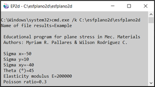
The educational application is run, and the name of the result file is assigned. Then, the input stress values required by the program are assigned, i.e., Sigma x= -50; Sigma y= 10; Sigma xy= -40; Theta (°) = 45, measured counterclockwise. To calculate the deformations using Hooke’s law, the values of Modulus of Elasticity E=200000 MPa and Poisson’s ratio ( =0.3 are provided, as shown in Fig. 4.
Once the input data is entered, the complete results of the plane stress problem calculation, including the associated deformations and strain energy density, are automatically displayed in a text file, as shown in Fig. 5.
Simultaneously, another window is displayed in MAXIMA with Mohr’s circle stress plot (see Fig. 6).


The Mohr’s circle of stresses in an enlarged view is presented in Fig. 7. The initial stress axis (xy), the rotated stress axis (x1y1), and the shear stress axis (ss*) are displayed in the plot of the Mohr circle. Also, are displayed the principal stress axis (s1s2), the double angle (2( ), the circle center, and the values of the stress points ((x,(xy), ((y,(xy), ((x1,(x1y1), ((y1,-(x1y1), the principal angles ((p1 and (p2) and the principal stresses s1 and s2, as shown in Fig. 7.
The usability test involved twenty-five engineering students from the Mechanics of Materials course at the Universidad Surcolombiana. The test was applied through classroom workshops using the computer application. At the end of the exercise, students were asked to rate on a qualitative scale of low, sufficient, satisfactory, high and excellent the following aspects:
The application’s usefulness in the subject context and engineering education (80% say excellent, 20% high).
The application contributes to learning plane stress and deformation (84% say excellent, 16% high).
The application adequately and completely solves the stress-strain problem with Mohr’s circle (100% said excellent).
The results are clear and complete (52% said excellent, 48% high).
In open questions, the students were also asked about the most outstanding aspects and those that should be improved. Among the most outstanding aspects, the following stand out: a) it is easy to use. b) it is a good assistant for solving exercises in class and for independent learning outside the classroom. c) it is reliable and safe. d) it presents the results quickly. e) it improves learning. f) Mohr´s circle is understandable, and the interpretation of results is easy. g) it presents the results for interpreting Mohr’s circle clearly and straightforwardly.
It was found that the most frequent aspect to improve was to add the values of the coordinates of the points in Mohr’s circle.
5. Conclusions and recommendations
An educational computational application was developed in Fortran and MAXIMA for the analysis of plane stress problems called EsfPlano2D, which assists in the step calculation of stresses, associated deformations, and strain energy and plots the Mohr’s circle of stresses. The results obtained through the development of the educational application show the feasibility of creating powerful and user-friendly tools tailored to the needs as a strategy to support the teaching-learning processes in the classroom and the accompaniment of ICT (Information and Communication Technology) for autonomous work at home.
The usability tests recognized the positive impact on teaching in the technological context of engineering students of the present century.
The application and the user’s manual can be requested at the authors’ e-mail addresses referenced in this paper’s title.
The simplicity and speed in the execution of stress and deformation calculations make the EsfPlano2D application an ideal tool for the execution of parametric studies involving failure studies.
It is recommended to continue exploring new possibilities to broaden the base of didactic computational tools in other topics of mechanics of materials.

