


 English (pdf)
 Article in xml format
 Article references
 Send this article by e-mail
 Cited by SciELO
  Cited by Google
  Similars in
SciELO
Similars in
SciELO  Similars in Google
 Permalink
1. INTRODUCTION
The analysis and estimation of the physicochemical properties of heavy oils such as density, viscosity, API gravity, and molecular weight, play a crucial role in the characterization of oil, and are necessary in upstream, downstream, and midstream activities of the hydrocarbon industry[1] . Although density is key to evaluate resources, viscosity is the property that most affects productivity and heavy oil recovery[2][3]. Moreover, these properties are directly involved in the optimization of oil refining operations, the determination and quality control of derivatives, the estimation of transport and storage conditions[4], the development of reservoir simulation processes[1], and the selection of a suitable oil recovery. However, measurements with conventional techniques take time, usually requiring tedious and expensive experimental processes, where accuracy decreases as oil viscosity increases, as equipment designs and protocols are focused on light and medium oils [5] [4] . Furthermore, human error in these measurements occurs more frequently and reflects a low reliability level in the characterization of oil, leading to failures in equipment designs for facilities, numerical simulations, and evaluation of reservoirs[6].
Low field NMR is proposed to overcome these difficulties. It is a novel technique that allows for indirect estimation of multiple properties of fluids, such as viscosity and density [7][8][9][10] [11], API gravity[12], molecular weight[4], aromatic content[6], total acid number and sulphur content[13], through mathematical models developed.
The success of LF-NMR measurements depends on the mathematical model. Several models have been developed to estimate oil viscosity and density using NMR spectra. For instance, Bryan et al. [21] developed a viscosity model from different reservoirs in Canada to estimate viscosity in the range of 1 to 3,000,000 cP for temperatures between 25 and 85 °C. In 2008, Burcaw et al. showed a correlation between the logarithmic mean of the transverse relaxation time (T 2gm ) and the hydrogen index (HI). The Burcaw model is suitable for oils with maximum viscosity of 107 cP. Vinicius (2014) developed a viscosity and °API gravity model using the transverse relaxation time (T2) and relative hydrogen index (RHI). The Vinicius model showed a good degree of reliability on 50 samples with viscosity ranging from 23.75 to 1801.09 cP and °API gravity from 16.8 to 30.6. Markovic et al (2020) related the viscosity with the Hydrogen index (HI) and the logarithmic mean of the transverse relaxation time (T2gm). The Marcovic model was developed with a suite of 23 Canadian heavy oils recovered from different reservoirs, with a wide range of temperatures (26-200 °C) and viscosity (70 -21,600 cP).
The required LF-NMR measurements are simple and nondestructive, capable of providing a large amount of valuable information about the fluids studied from a small sample [7][9] [14]. In addition, the LF-NMR technique offers the possibility of performing either laboratory or in situ measurements with borehole logging tools, making this a more attractive technique[15][16]. However, LF-NMR measurements depend on the oil properties and the details of data acquisition[9] [17]. Moreover, the above models have default parameters derived for heavy oils from a certain field and, when applied to different heavy oils, considerable prediction errors[18]occur. Hence, the models must be customized for each NMR equipment and fluids group.
Therefore, for purposes of this research, the mathematical models proposed in literature were evaluated to estimate the density and viscosity of heavy oil by low field NMR. The main objective was to adjust the selected models to properties of a Colombian heavy oil and to show the LF-NMR quantitative and qualitative abilities as compared with conventional techniques. The tuned models and the comparison study will be a starting point to extend the use of the NRM technique to other Colombia heavy oil with a low uncertainty level.
2 EXPERIMENTAL DEVELOPMENT
In this section the workflow to evaluate the NMR models in literature and to determine the density and viscosity of the mixture toluene and Colombia heavy oil (Figure 1) is explained.
OIL-SOLVENT MIXTURES PREPARATION
Toluene was selected as liquid solvent due to its dilution efficiency and capability of interfering in asphaltene aggregation processes and producing homogeneous mixtures with heavy oil. For preparing the samples, Colombian heavy oil (12 °API and water content <1%) and toluene were combined to obtain a mixture with a solvent concentration of 0%, 2%, 4%, 6%, 8%, 10% y 12% m/m. These proportions were selected to achieve properties similar to those of heavy oil, i.e, the viscosity range was between 100 and 10,000 mPa.s and the gravity was between 22.3 and 10 ° API[19].
Initially, the heavy oil sample was thermalized in an electric oven for hours and then poured directly into a flask to prepare the mixtures with toluene. Next, the oil-solvent samples were shaken for 3 hours and then heated at 40°C. Finally, the blends were transferred into NMR tubes.
NMR ANALYSIS
The mixtures were characterized using a Bruker relaxometer of the Minispec mq series, with a frequency of 7.5 MHz. The samples were stabilized at 40°C, which is the equilibrium temperature of the magnet bore.
The Car-Purcell-Meiboom-Gill (CPMG) pulse sequence was used to determine transverse relaxation time (T2). The acquisition parameters of the equipment for the CPMG pulse sequence were: 5000 echoes, 32 scans, 0.5 ms between echoes and 15 s recycling, for a mass of 6 g per sample. The Inverse Laplace Transform (ILT) was applied to the NMR measurements to invert the multi-exponential decays, and to obtain the T2 distributions with the dynamics center software.
VISCOSITY AND DENSITY DETERMINATION
The viscosity and density of the samples were determined in a conventional way with a Stabinger 3001 viscometer from Anton Paar at 40°C, under ASTM D7042 standard [20]. The repeatability and reproducibility percentages reported by the standard were 0.1% and 0.54% for viscosity and 0.03% and 0.14%. for density tests.
NMR MODELS EVALUATION
The NMR models with default parameters found in the literature, were used to estimate viscosity and density with the NMR results obtained in each test. The values determined were compared with the information from Stabinger 3001 by error calculations. When the error values were significant, the NLS regression was performed to tune the NMR model and thus achieve optimal values for their empirical constants (Figure 1).

For viscosity measurements, the NMR models accuracy was assessed visually on linear regression plots and by comparing coefficients of determination - R2. Moreover, the root mean square error (RMSE) and the maximum absolute error (MAE) of the predictions were calculated as statistical metrics, due to the wide range of viscosity in existing research (Table 1). The MAE represents the largest absolute difference between predicted and observed viscosity values. The RMSE is the square root of the differences between predicted values and observed values or the quadratic mean of these differences. As for density, the parameter selection was based on the lowest percentage of relative error due to its small-scale values (Table 1).

3. RESULTS AND DISCUSSION
VISCOSITY AND DENSITY ESTIMATION WITH CONVENTIONAL METHODS.
Table 1 summarizes the estimated experimental results by the Stabinger viscosimeter as a conventional method. The measurements of the eight (8) samples represented the real value, which was used to calculate the error percentages and the deviations of the obtained values with LF-NMR.
Figure 2a shows a linear dependence between the density and the amount of toluene, indicating that for each gram of toluene added the density decreases by approximately 0.0011 g / cm3 at a temperature of 40 ° C

On the other hand, Figure 2b shows the magnitude of the reduction in viscosity due to the addition of this solvent. It is observed that by adding a small amount of toluene, there is material reduction of viscosity. However, the viscosity reduction percentage is lower at a higher toluene concentration. Hence, it allows to ensure that in the dilution process, the solvent efficiency is not proportional to the amount of solvent, since at a solvent added concentration greater than 12%, the viscosity reduction is not meaningful.
NMR PARAMETERS ANALYSIS
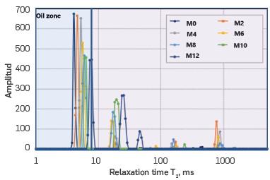
The results obtained from NMR are distribution curves, as those shown in Figure 3. The distribution curves relate the amplitude with relaxation time T2 and show different behaviours in each sample analysed. The relaxation time distribution of Figure 3, suggests that as the amount of toluene added increases, the amplitude of the mixture decreases in the oil zone, i.e. at T2 less than 10 ms[11], and towards the right region of the relaxation distribution, the amplitude of peaks that represent the light fractions raise.
Before estimating the properties of the fluids with NMR, it was necessary to analyze the relationship of the NMR parameters (RHI and T2gm) with conventional density and viscosity measurements to select the most appropriate model.
First, the geometric mean of T2 (T2gm) was estimated, using equation 1 and the information of Figure 3:

Where:
T2gm: The geometric mean of T2
Al: Amplitude for each T2i
T2i: Relaxation time of each point.
Next, the Amplitude Index (AI) was calculated:

The amplitude index allowed to calculate the Relative Hydrogen index (RHI). The RHI provides information on the amount of hydrogen in a sample with respect to the amount of hydrogen in a water sample, by relating the amplitude index of the sample (Al sample ) with the water amplitude index (Al water ) through equation 3.

The relationship of the NMR parameters with the viscosity and density are presented in Figures 4 and 5, respectively.


The first analyzed NMR parameter is relaxation transversal time. T2 increases as the function of viscosity decreases, as reported in the literature [11][7]. As shown in Figure 4a, a mixture with a high viscosity (low concentration of toluene) tends to have a very small T2, due to the high molecular weight and the closeness of its molecules, relaxing very fast. Likewise, Figure 4b shows that the Relative Hydrogen Index raises as viscosity decreases, as the amount of hydrogen becomes higher as the solvent concentration increases in the mixtures.
Further, Figure 5 presents the relationship between density and NMR parameters. The first analyzed parameter was T2gm (Figure 5a), where its value increased by decreasing the density in the samples. Therefore, the relaxation time values increased, when the number of light compounds (hydrocarbon) raised in the mixtures. As regards the Relative hydrogen Index (RHI) in Figure 5b, as solvent concentration and the mixture density increased, the content of hydrogen atoms in the sample and the amplitude values decreased.
Then, a multivariable regression was performed to relate the viscosity and density from the information obtained with the NMR relaxation times distributions through an ANOVA analysis. The results show the Pvalue estimated for the density and viscosity model with a significance level of 5% as 0.0003 and 0.0006, respectively (Equations 4 and 5). Those values confirm a statistically significant relationship between the NMR parameters (RHI and T2gm) and the fluids properties evaluated.

Finally, the figures and trends evidenced the strong relationship between the viscosity and density with RHI and T2gm, such as the models shown in the literature to evaluate the properties of heavy oils and mixtures [12][9][8][21][7][10]. However, the models are not universally applicable. They can be affected by the magnetic field of the equipment, the acquisition parameters, and the fluid properties [9]. These have been adjusted mainly to Canadian heavy oils and specified NMR equipment features. Hence, the model constants must be customized for a Colombian heavy oil and the NMR equipment used in this research, as a first step in the characterization of Colombian fluids with LF-NMR.
VISCOSITY ESTIMATION BY NMR
Based on the relationship between viscosity and NMR parameters, the models with the T2gm and RHI were used as input parameters. The models are listed in Table 2, with the number of fitting (free) parameters and recommended conditions. Where:

η: Viscosity (Cp)
RHI: Relative hydrogen index (ad)
T2gm: The geometric mean of T2 (ms)
HI: ρo/ρw *RHI
ρo , ρw= oil and water density (g/cm3)
First, the Bryan model [21] was studied. To choose α and β constants, the values reported by Bryan et al. [21]. Wen et al., [7], Bryan et al. [11] are listed in Table 3 Next, each value was used to calculate the viscosity, and the constants with lower error were used to analyze the model.
Table 3 Experimental values of α & β found in the literature for heavy crude oils diluted with solvents.

The best fit was achieved through the set of data S8 that corresponded to the values 1749 and 4.69 for a and (3, where MAE, RMSE and determination coefficient (R2) were 40.96 cP, 73.07 cP and 0.99, respectively (Figure 6 and 7). Despite the good match with the selected parameters, the NLS linear regression was considered to reduce the error (Figure 6a). The results present that the best fit is achieved with a and (3 values of 1834.85 and 4.6 respectively. The MAE and RMSE were slightly reduced to 35.02 mPa.s and 65.06 mPa.s after regression, as it is depicted in Figure 7.

Figure 6 Rheological viscosities compared to NMR viscosities of 7 samples. Solid black line (1:1) presents a perfect prediction for all models.
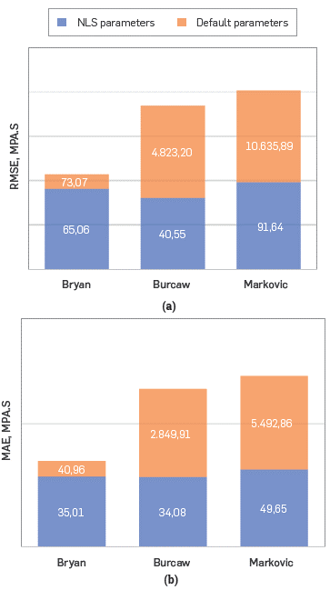
Figure 7 Compared (a), Root-MSE (b) and MAE of NMR model predictions for using three model configurations. Bryan (2003), Burcaw (2007) and Markovic (2020)
For the Burcaw [9] and Marcovik [8]model only one set of data for the fitting parameters was found in the literature (Table 2). Nevertheless, with these parameters scattered data (Figure 6a. blue points) , high MAE and RMSE were obtained for both models (Figure 7). Figures 6b and 6c show that most predictions did not fall within a factor of one (solid black line).
Therefore, it was necessary to use the NLS regression with the GRG nonlinear method to determine optimal parameters for the 7 samples. For the model Burcaw, the results showed that the lowest MAE and RMSE were reached with m and s values of 13.68 and 6.54, respectively (Figure 5a red points). Likewise, for the Marcovik model, the best values to a, b, c and d were 1084.2, 5.16, 10031.2 and 2.3, respectively.
Figure 7 shows that Burcaw [9] and Marcovic [8] RMSE and MAE values were several times lower after tuning the parameters. Moreover, most predictions fall within a factor of one and the determination coefficients (R2) were 0.997 and 0.998, respectively (Figure 6b and 6c).
Vinicius model [12] model was not analyzed due to the properties of the fluids and given temperature conditions, as this mathematical expression is valid for viscosity ranges between 23.75 cP and 1801.09 cP, and RHI values of 0.94 and 1.18 at 27.5 °C.
The most accurate prediction was reached with the Burcaw model in the conditions given, but only after the NLS regression. In comparison with Bryan et al. and Markovic et al., Burcaw et al. had a 24.52 mPa.s and 51.09 mPa.s lower RMSE score, respectively, while the MAE score was 0.93 mPa.s and 15.57 mPa.s lower, respectively.
Bryans model could also be a good option to determine the viscosity of heavy oil with toluene since it showed a slightly higher error (RMSE and MAE) as compared with the Burcow model.
It showed a good fit with the properties of Colombian heavy oil and the NMR equipment specifications, even before NLS regression, by using literature parameters. Therefore, this model can be used when there is not enough data on viscosity.
DENSITY ESTIMATION BY NMR
The correlation proposed by Wen et al (2005) was used for density estimation. The Wen correlation shows an inversely proportional relationship between the NMR parameters (IA and T 2gm ) and density as per equation 6. The constants A and B were chosen from the values listed in Table 4. The constants selection was based on the lowest percentage of relative error (ε).

According to the tabulated data (Table 4), the lowest error percentages are reflected on the set of data number 2, where A= 1.0373 and B=0.0117.

Figure 8 shows the graphical analysis of the results, where conventional density is compared with the value acquired by NMR. From the numerical study, a coefficient of determination of 0.96 and a linear relationship with a slope of 1.057 were obtained. These values reflect the low percentage of error obtained and the high degree of precision of the Wen correlation.

QUALITATIVE COMPARISON OF TECHNIQUES
The quantitative results prove that NMR is a reliable and accurate technique to evaluate oil viscosity and density based on mathematical models with acceptable errors, based on mathematical models. In addition, NMR is an alternative offering several qualitative advantages. Table 5 shows a comparison between conventional techniques used in this investigation and the NMR technique.

The above comparative study shows the operational factors advantages that help overcome the issues related to common human errors and protocols when heavy oil is measured. Furthermore, density and viscosity models in literature have a wide range of application from light oils to extra heavy oils, with low prediction errors, provided that the parameters are correct. Moreover, the LF-NMR technique offers the possibility of conducting measurements, either at the lab or in situ, with borehole logging tools.
CONCLUSIONS
 This study evaluated and adjusted some mathematical models to estimate the viscosity and density of a Colombian heavy oil through LF-NMR. The best option to represent the viscosity was the Burcaw model, but only after the NLS regression, with RMSE and MAE values of 40.55 cP and 34.08 cP, respectively. On the other hand, the Wen correlation was preferred to determine density with a relative error of less than 1%, while the determination coefficient was 0.96.
Bryans model is a good option when there is not enough data available on viscosity to determine the fitting parameters trough NLS regression. Because those found in the literature showed a good fit with the properties of Colombian heavy oil and the NMR equipment specifications. In addition, the acquired RMSE and MAE were slightly higher than the Burcow model.
The comparison of both measurement techniques shows that low-field NMR is better than the conventional technique, as this technique helps overcome the issues to determine viscosity and density in heavy oil. It is worth to note that it offers multiple advantages as to operational and measurements factors, such as wide range for accurate density and viscosity measurement, a shorter test execution time, minimum required sample volumes with 100% recovery, and no need for tedious cleaning procedures between measurements.

