


 English (pdf)
 Article in xml format
 Article references
 Send this article by e-mail
 Cited by SciELO
  Cited by Google
  Similars in
SciELO
Similars in
SciELO  Similars in Google
 Permalink
Introduction
The downward continuation of the potential field can provide abundant information on the spatial distribution of the potential field and is an important part of the interpretation of gravity and magnetic anomalies (Zhu, Cao, & Lu, 2014; Deng, Liu, Song, & Chen, 2014). Luan Wengui adopted another regularization functional and deduced another response. According to the same regularization functional, another response formula was derived by Luan Wengui, which is suitable for understanding the distribution characteristics of the source potential field in the near field (Zhang, Dai, & Liu, 2014). C. W. Groetsch, P Mauriello, D Patella, Xu Deshu, Zeng Hualin, Wang Xuben, Gao Yongcai and other scholars have also studied the extension method. Through research and comparison, it shows that the regularization method has the best downward extension effect. But due to the influence of the Gibbs effect, on both sides o.Vie main anomaly zone, there is often a "positive and negative alternating " " shaped weak anomaly zone with the main source distribution area as the center, which may be a separate anomaly or composite anomalies formed by the superposition with other anomalies, thus increasing the difficulty to explain the field source. To solve this problem, based on the gravity and magnetic data regularization downward extension, this paper puts forward downward gravity and magnetic property parameters inversion method of downward continuation and anomaly separation based on the iterative method, providing a new way of thinking for the comprehensive interpretation of the field source from the material properties and geometric parameters (Al Farajat et al., 2015; Li & Zhang, 2017; Mazgaj, Szular, & Szczurek, 2017).
Regularization extension technique
According to the Laplace equation and the boundary condition of the potential field, there is:

U (x, z) is the potential field at the measuring point (x, z),and f (x, z) is the known field value on the measuring point; Ф (x) is the height of the measuring point. By using the method of separating variables and the boundary condition, the general formula of the series decomposition of the field potential can be obtained (Boehm & Ulbrich, 2015).

Set M as the number of points at the measuring point, and ∆x is the distance between the measuring points, there are
This result is the series decomposition method of the traditional downward continuation (Raknes & Arntsen, 2014).
In order to overcome the oscillatory effect, the series is still taken as the basic form of the field value solution. In solving the continuation function, a decomposition function with a relatively smooth variation is selected and the error of fitting it to the original field is minimized on the original observation profile, so that the analytical function of regularized downward continuation series after correction can be obtained (Zhang et al., 2015; Fontchastagner, Lubin, Mezani, & Takorabet, 2018).

v
i
. is called the regularization factor, which is
 ,a function related to the frequency λ
i
., continuation depth z and coefficient α. It corrects the frequency of the series term of the continuation field, and it is proved by practice that as long as the regularization function is properly selected, it cannot only guarantee the non-singularity of the potential field in the process of continuation, so as to obtain the complete field value distribution in the lower half space, but also the Gibbs effect cannot be very significant.
,a function related to the frequency λ
i
., continuation depth z and coefficient α. It corrects the frequency of the series term of the continuation field, and it is proved by practice that as long as the regularization function is properly selected, it cannot only guarantee the non-singularity of the potential field in the process of continuation, so as to obtain the complete field value distribution in the lower half space, but also the Gibbs effect cannot be very significant.
Iterative continuation technique
It is often necessary to extend downwards to the top of different depth layers to separate the anomalies produced by different depth layer sources on the ground. The stability and depth of continuation directly affect the result of continuation. To deal with the instability of potential field downward continuation and the limited depth of downward continuation by the classical FFT method, Xu Shizhe put forward a downward continuation method in spatial domain, which is implemented based on stable FFT upward continuation. The principle is simple and the downward continuation is stable. The basic idea of the downward continuation of the iterative method is to assume that there are two planes, ГA and ГB, representing the ground surface and the plane of a certain depth under the ground, respectively. Between the two, there is no field source distribution, that is, there is a passive space, so that the downward continuation iterative solution ofthe known depth based on upward continuation can be realized according to the following diagram (Chen, 2015).

Inversion of physical parameter of gravity and magnetic anomaly
Assuming the thickness of a certain depth of the underground layer as h, the layer is divided into MN(MN = M X N) small vertical prisms of the same size with a finite extension, and the coordinate of the center point of the small prisms is (x 0j , y 0j ) and residual density is ρ j (j = 1,2,3,---, MN) ; its side length is α and b respectively; the top depth of the prism is h and the height is dh. Thus, the formula for the frequency spectrum ḡ j (u, v) of the gravity anomaly g j (x, generated by the ground (x,y) of each prism in the frequency domain is as follows:

In the upper formula, u, v represent the wave number of x, yrespectively; G is the gravitational constant; and
 . The frequency spectrum ḡ (u, v) is made Fourier inversion to obtain the gravity anomaly g (x, y) in the space domain.
According to the superposition property, the frequency spectrum ḡ (u, v) of gravity anomaly g (x, y) produced by the whole depth layer at the ground (x,y) isas follows:

Formula 5 is the forward formula of field source gravity anomaly with known physical parameters.
If the gravity anomaly g(x, y generated by the depth layer in the top surface is known, h = 0 (if h ≠ 0, that is, the buried depth is not zero, and it can be extended to the top interface first, and then:

Thus:

The following formula can be deduced from the above:
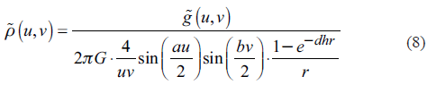
Thus, by Fourier inverse transformation, the residual density values of each point (x, y \ on the top surface of the depth layer can be obtained:

Formula 9 is the inversion formula for calculating the relative physical parameters of the gravity anomaly of the known field source. The apparent density corresponding to the gravity anomaly can be calculated by the formula.
For the magnetic source anomaly, the gravity anomaly of the magnetic source can be obtained first, and the magnetic source density or magnetization intensity can be inversed by the same method. In view of the space, its calculation formula is not deduced in this paper.
Regularized continuation depth constrained inversion of single model gravity and magnetic anomalies
In this paper, a 101 x 101 mesh is designed, the distance between points and that between lines is all 1 (unit: meter), that is, the measuring area is 100 x 100m2. The specific parameters of the sphere model are shown in Table 1.
Table 1 Specific parameters of a single sphere model
| Spherical center coordinate (m) | Sphere radius (m) | Residual Density (g/cm3) | Magnetization intensity (A/m) | Magnetization inclination | Magnetization deviation angle |
| (50,50,20) | 5 | 0.5 | 100 | 45° | 0° |
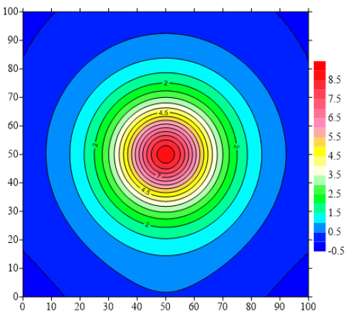
The corresponding gravity anomalies (∆ g) and magnetic anomalies (∆ T) are derived from the forward calculation of the above model, as shown in Figure 2:

Figure 3 is a section of the regularization result of the above magnetic anomalies, which shows that the center of the anomaly is consistent with the depth of the given model. However, due to the influence of the Gibbs effect, on both sides of the main anomaly zone, there is often a "positive and negative alternating "
 " shaped weak anomaly zone with the main source distribution area as the center, which may be a separate anomaly or form composite anomalies by the superposition with other anomalies, thus increasing the difficulty to explain the field source.
Regularization continuation depth constrained inversion of superimposed gravity and magnetic anomalies
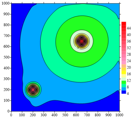
In order to carry out theoretical calculation and verification, a 201 x 201 mesh is designed in this paper. The distance between points and that between lines is all 5 (unit: meter, that is, the range of measuring area is 1000 x 1000m2. The model consists of three vertical prisms, in which the column centers of model 1 and model 3 are on the same vertical line, and the specific parameters of each column model are shown in Table 2:
Table 2 Specific parameters of the combined model
| Parameters cylinder | Cylindrical center coordinate (m) | Cylinder length (m) | Cylinder width (m) | Cylinder height (m) | Density (g/cm3) | Magnetization intensity (A/m) | Declination | Magnetic dip |
|---|---|---|---|---|---|---|---|---|
| 1 | (650,650,500) | 300 | 300 | 100 | 0.4 | 80 | 0° | 45° |
| 2 | (200,200,50) | 50 | 50 | 50 | 0.5 | 100 | 0° | 45° |
| 3 | (650,650,50) | 50 | 50 | 50 | 0.5 | 100 | 0° | 45° |
According to the relevant parameters of the above model, the gravity anomaly and magnetic anomaly (unit: nT) of the model can be obtained by forward modeling (unit: mGal). The result is shown in Figure 6.
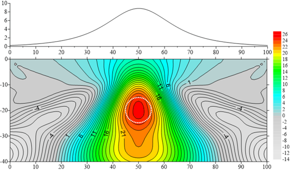
Figure 4 The principal curve of magnetic source gravity anomaly and its regularization downward extension fracture surface

Figure 5 Magnetic source gravity anomaly (left) and apparent density inversion results (right) (a) Spatial position of the model (b) Model plane position and parameters

In order to extend this method to the processing of magnetic anomalies effectively, the magnetic anomalies' magnetic source gravity is solved first, and the magnetic anomalies are also solved according to the gravity anomaly process. Figure 7 shows the magnetic source gravity anomaly of the magnetic source model.


Figure 8 Anomaly curve of diagonal section of magnetic source gravity anomaly and its regularized extension
The anomaly of the main section of the model is selected for regularized downward continuation, so that the depth of the field source is obtained respectively. It can be seen from the diagram that the depth of the regularization extension has a high accuracy.
The regularization is used to establish the depth of the field source for iterative continuation. Considering that the basic requirement of iterative continuation is that the two depth interfaces are passive field spaces, the idea of this paper is to carry out the continuation of shallow source depth first; then, the shallow-source anomaly is separated by cutting method, and the cutting radius is established according to the anomaly range of shallow-source anomaly. (the idea of this paper is to use Laplace operator to establish abnormal boundary and then the radius is taken as (L+D)/2) according to the anomaly boundary.)


Conclusion
Based on the potential field theory and regularization theory, a method for inversion of gravity and magnetic physical property parameters of downward continuation and anomaly separation based on iterative method is proposed. The following points should be pointed out:
1) The inversion effect based on single model depth constraint is better;
2) The lateral superposition model can obtain higher lateral resolution anomalies in the process of iterative downward continuation. Therefore, the inversion of physical parameters has a higher accuracy, while the vertical superposition anomaly and physical properties are related to the separation accuracy of anomalies.
3) The study of high accuracy anomaly separation is the key to the inversion of depth constrained physical parameters of complex geological models.

