


 English (pdf)
 Article in xml format
 Article references
 Send this article by e-mail
 Cited by SciELO
  Cited by Google
  Similars in
SciELO
Similars in
SciELO  Similars in Google
 Permalink
1. Introduction
The design of antennas is a complex process that requires running electromagnetic simulations and depends on many variables that affect the bandwidth, losses, and gain of the antenna. Therefore, it is appropriate to apply optimization techniques to obtain the best results for a particular objective [1,2]. However, a small percentage of the antennas recently published in the literature are designed by means of optimization to determine the size of their structure, which allows enhancing the optimal search according to the design premises of the selected application [3].
The optimization methods employed in recent years for the antenna design are Genetic Algorithms (GA), Particle Swarm Optimization (PSO), Surrogate-Based Optimization (SBO), and Fractional Factorial Design (FFD). The GA, PSO, and SBO methods are heuristic, and they are based on the individual experiences or surrogate models, to resolve design problems; whereas FFD is a probabilistic method based on the variance analysis for determining the optimal solution [3].
Among these methods, PSO is one of the fastest heuristic approaches for finding the optimal solution of a complex problem [4]; it is considered an artificial intelligence method. Therefore, it has been applied in multiple antenna optimization processes to reduce computation time by preventing next particle generations from being equal to previous iterations [5].
PSO has been applied in many different fields, and several variants have been proposed with the modification of some of its parameters or steps for improving performance. For example, when a particle does not improve its result, it is helpful to intervene on it, so the algorithm can find the optimum faster. Also, the combination of different optimization techniques with PSO can enhance performance for particular applications [6].
Regarding antenna optimization, some of its variants are: hierarchical PSO to enhance search space exploration, a self-organizing hierarchy with time-varying acceleration coefficients [7]; neighborhood-redispatch PSO to avoid the premature convergence problem with a global search strategy through the inclusion of factors that modify the calculation of updated velocity [8]; PSO with velocity mutation to apply a mutation in the velocity of particles that do not improve its result at a given time [9]; and quantum-behaved PSO to reduce the number of controlling parameters where particle movement is described by the probability density function in terms of the wave function [10].
In the research works described above, different variables were optimized, including beam width [7], bandwidth, considering the standing wave ratio [8-10], and gain [9], in order to obtain the best performance according to the design premises. In any case, it is a priority to obtain the best performance in the desired bandwidth, which can also be done by achieving the lowest S 11 magnitude possible to reduce the return losses produced by the matching impedance with the communication system; for example, in [11,12], the authors applied PSO to optimize this parameter.
In this work, we present a new modified PSO method with a strategy based on the intervention in the global search for the worst particles, i.e., the particles that do not improve their response. This modification aims to enhance the performance of conventional PSO in terms of the search for the optimal solution, as well as to reduce the number of iterations needed. The proposed method is applied to benchmark functions and antennas of narrowband and ultra-wideband to validate its operation. The objective function for the optimization is based on obtaining the lowest S 11 magnitude in the desired operating frequency range.
2. Description of the proposed modification for the method of optimization
In this section, the conventional and modified methods of optimization are explained, describing their algorithms, equations, and parameters to resolve problems with real and binary variables.
2.1 Conventional particle swarm optimization
The conventional PSO algorithm is shown in Fig. 1, and its parameters are the following: N is the number of dimensions (real and/or binary); M is the number of particles; Niter is the number of total iterations; w is the inertial weight; c1 and c2 are cognitive and social parameters; η1 and η2 are random values for each particle and iteration; and V n max represents the maximum velocity for each dimension calculated with eq. (1), where Xn max is the maximum position, and Xn min is the minimum position of dimension n [13].


The convergence criteria are that the number of iterations (N iter ) must be equal to a determined maximum number, and that the best value of particle must not change in a consecutive number of iterations N cons iter When any of these two conditions is accomplished, the optimization process ends, and the best position of the swarm is obtained [14].
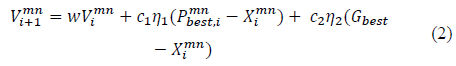
To update the velocity of particle m and dimension n, eq. (2) is employed, where the value of the best response of the particle is P mn best,I for each iteration i and particle m; the best response of the swarm is G best , and the position of the particle m, dimension n, and iteration i is X mn i This value must be between a maximum (V n max ) and a minimum (-V n max ) [14].
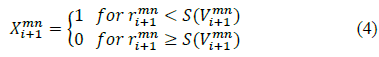
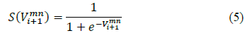
The updated position for real dimensions is calculated through eq. (3), and it must be in a confinement interval between Lim n min and Lim n max [13].Meanwhile, eq. (4) is used for the binary dimensions, where S is the probability that a particle can change its state to a logical one, and r i+1 mn is a random value in the range between 0 and 1. With that expression, a binary value (0 or 1) is obtained for each particle, which is discretized through the Sigmoid transformation in eq. (5) [15].

2.2 Modification of particle swarm optimization through the intervention technique
The modified Particle Swarm Optimization with Intervention Technique (PSOit) proposed in this work is based on following the best particle of the swarm. When any particle does not improve its result for a previously determined number of iterations, it is intervened, so it is attracted to the best particle and guided toward the region with more potential for improvement.
Therefore, the intervened particle has the opportunity to benefit from the global experience of the swarm and can increase the speed of convergence of the algorithm. This intervention ends when the response of the particle improves. Then, the conventional method is applied to this particle until the conditions for another intervention emerge.
In Fig. 2, a 2D parameter space acceleration diagram is presented to exemplify the proposed modification, it shows the acceleration of particles toward the location of the best response of the particle and the best response of the swarm using conventional and modified methods. In Fig. 2(a), the velocity of particle 1 in the next iteration (i+1) keeps pointing toward its best response, which is away from the region of the best solution of the swarm. However, Fig. 2(b) shows that the velocity of particle 1 (intervened particle) in i+1 is moving toward the best response of particle 3, which is the best particle from the swarm. Therefore, the intervention allows obtaining an acceleration toward the region with more potential for improvement, thus leading to a better response from particle 1.

Source: Authors.
Figure 2 Diagram of acceleration toward the location of the best response of the particle and the best response of the swarm for particles 1, 2, and 3 with conventional (a) and modified (b) methods in a 2D parameter space.
In this way, the PSOit aims to improve the performance of the swarm. The proposed algorithm is shown in Fig. 3, where the modifications to the conventional algorithm are marked in gray. The conditions for applying the intervention are as follows: that the number of iterations without change (𝑁 m unchanged) is larger than 1; and that the intervention factor of the particle m (Interv m ) is larger than the random decision factor, whose characteristics are explained in Section 3.2.

The intervention factor of the particle is calculated with eq. (6), where the sum in the denominator goes from 1 to M-1 because the number of iterations without change from the best particle is excluded to prevent the modification from being applied to that particle. If both aforementioned conditions are met, the particle is intervened, which means that its updated velocity is determined through eq. (7), instead of using eq. (2), which is applied if there is no intervention.


3. Performance of PSOit with benchmark functions
To evaluate the performance of the proposed modification, six benchmark functions were used in the optimization with PSO and PSOit, four of them with real dimensions and two with hybrid (real and binary) dimensions. The methods were programmed using Matlab, on a PC with an Intel Core i7 2.4 GHz processor and 8GB RAM. The size of the population was 20 particles, the maximum number of iterations was 1000, and each benchmark function was optimized 100 times.
The rest of the parameters of the methods were configured as follows: for the real dimensions, the inertial weight was between 0.9 and 0.4, the cognitive parameter was from 2.8 to 2.0, and the social parameter was between 1.2 and 2.0 during the optimization time. Also, η1 and η2 were random values between 0 and 1 [16]. For the binary dimensions, the inertial weight was constant and equal to 1, the cognitive and social parameters were constant and equal to 2, and the maximum velocity was 6 [17].
3.1 Benchmark functions
The benchmark functions were: eq. (8) (Schaffer's F6), eq. (9) (Rastrigin), eq. (10) (Rosenbrock) [14], eq. (11) (Ackley), eq. (12) (Alpine) [13], and eq. (13) (Schwefel) [8]. These functions were tested with the conventional and modified PSO algorithms for minimization problems with the characteristics shown in Table 1, where the type and number of dimensions of each function are also detailed. For the evaluation of the hybrid algorithms with the benchmark functions (whose inputs are originally real dimensions), the binary dimensions were mapped to the real search space using eq. (14) [17].


3.2 Selection of the decision factor distribution parameters
The decision factor for the proposed method is a random number with a normal distribution, which was selected because its values are balanced around its mean. To select the mean of the distribution, three different values were evaluated (0.25, 0.50, and 0.75) to determine the best results. Also, the selected standard deviation (σ) was 0.1 to concentrate the random values near the mean parameter.
Table 2 shows the results of the mean and standard deviation of the global best responses from the benchmark functions after 100 repetitions, which were obtained through the optimization with PSO and PSOit for the different mean values of the distribution. In these cases, the PSOit method’s performance was similar or better than PSO for the three mean values, and the mean equal to 0.25 had the best results, i.e., it reported the lowest mean and standard deviation of the global best response for all the benchmark functions.

Table 2 Results of the objective functions with the process of optimization from the PSO and PSOit with a normal distribution (σ = 0.1).

Source: Authors
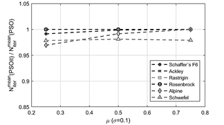
Additionally, Fig. 4 shows the results of the benchmark functions obtained with PSOit, normalized in terms of the response of the conventional PSO for different means of the decision factor distribution. It is noted that the normalized responses with a mean value of 0.25 had a reduction between 4 and 24.4% in comparison with the PSO responses. PSOit showed a better quality of solution than the conventional PSO with these parameters.

Source: Authors.
Figure 4 Normalized values of the mean benchmark functions for the normal distribution with different a mean and a standard deviation of 0.1.
Regarding the number of iterations, the proposed method had a similar performance to the conventional PSO for meeting the convergence criteria (Table 3) in the global best response, where the distribution mean of 0.25 had the best results.
Table 3 Results of the number of iterations with the process of optimization from the PSO and PSOit with a normal distribution (σ = 0.1).

Source: Authors.
Fig. 5 shows the average number of iterations for the PSOit, normalized in terms of the average number of iterations of the conventional PSO for the different distribution means of the decision factor. It is noted that the average number of iterations decreased by 4%, which means that PSOit allows reducing the number of iterations and evaluations of the objective functions to accomplish a better global response of the swarm in comparison with the conventional PSO.
Source: Authors.
Figure 5 Normalized values of the mean number of iterations for the normal distribution with different decision factor distribution mean and a standard deviation of 0.1.
Considering the above, PSOit has the best performance using a normally distributed decision factor with the following parameters: 0.25 (mean) and 0.1 (standard deviation). This means that the intervention should be applied to the particle in a low number of iterations without change, guiding it toward the region with better response and preventing it from being lost in the search space.
4. Application for antenna optimization
The proposed method was applied in the optimization process for the design of three different antennas, in order to uphold its advantages in comparison with the conventional PSO for the search for optimal solutions in this field. The selected designs were one narrowband and two ultra-wideband printed rectangular microstrip antennas (PRMA). Both shape and hybrid optimization were applied in these designs.
To conduct the simulation of the proposed method in antenna design, an optimization environment was implemented, as shown in Fig. 6. In this environment, Matlab was employed for applying the optimization algorithms (PSO and PSOit), and the HFSS API by Ansoft was employed to integrate the electromagnetic simulations in HFSS with Matlab [18]. Visual Basic code was implemented to create and run the HFSS simulation and import the corresponding results to Matlab.

4.1 Wi-Fi antenna at 2.45 GHz
The first antenna design was a PRMA for the Wi-Fi communication system at 2.45 GHz, with a conventional structure and microstrip feeding method (Fig. 7), which has been one of the most implemented for this kind of system, due to its good performance and adaptability. The selected substrate was the FR4-epoxy, given its high electrical permittivity, which reduces the size of the antenna in comparison with other conventional materials [3], and whose characteristics are as follows: a thickness of h=1.6 mm, a relative electrical permittivity Ɛr=4.4, and a loss tangent tan(δ)=0.02.

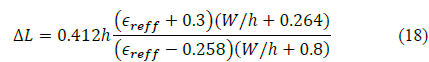
In this experiment, the control variables for optimization were the length and width (L and W, respectively) of the antenna’s resonant patch. The selected lower and upper boundaries for these variables were 8.8 mm ( L ( 48.8 mm, and 7.3 mm ( W ( 67.3 mm. Furthermore, the size of the feeding microstrip was kept constant and equal to a quarter of the wavelength. The calculated initial variables were L= 28.8 mm and W = 37.3 mm. These values were obtained through eq. (15), (16), respectively, where λL is the wavelength of the minimum frequency, ϵreff is the effective relative electrical permittivity that is defined by eq. (17), and ΔL is a distance according to eq. (18) [19].


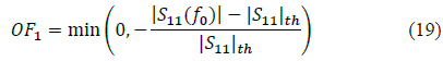
The objective function that allows the minimization of the S 11 magnitude in the central frequency was eq. (19), where |S 11(f 0)| is the S 11 magnitude at the central frequency f 0=2.45 GHz, and |S 11|th is the threshold magnitude equal to -10 dB [20]. The maximum consecutive number of iterations for the convergence criterion was 80 [14].
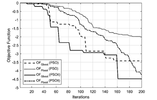
Results obtained for the global best response (Gbest) and the mean of the best response of all the particles (Pbest) as a function of the iterations are shown in Fig. 8 for the conventional and modified methods. It is worth noting that PSOit presented better results than PSO both for Gbest and Pbest during the optimization process. In this case, the proposed method improves the search of the global best through the intervention technique, thus obtaining a final optimal response equal to -4.479, while the result was -3.420 with the PSO.
Source: Authors.
Figure 8 Objective function according to the iterations for the optimization of a Wi-Fi antenna with PSO and PSOit.
Regarding the performance of the antenna, as expected, both optimization methods improved the initial calculated design. The S 11 magnitude at the central frequency was equal to -54.79 dB with the implementation of PSOit, while it had a value of -44.20 dB with the conventional method, as is shown in Fig. 9. Therefore, this is a demonstration of how the application of PSOit for the optimization of a PRMA for Wi-Fi at 2.45 GHz allowed obtaining a better response, thus improving the impedance matching of the antenna and reducing the reflection loss.

4.2 Ultra-wideband (UWB) antenna
The second application design was a conventional UWB PRMA, as shown in Fig. 10. The UWB PRMA has been widely used for enabling the joint transmission of several wireless communication systems. The design frequency range (where |S 11| ≤ |S 11|th) was established from 1.7 to 3.7 GHz to receive GSM, UMTS, LTE, WLAN/ISM (2.4 GHz), WiMAX, and 5G (3.5 GHz) communication systems with a threshold equal to -10 dB.

In the same way as the first design, a microstrip was employed as a feeding method [3], and the substrate was the FR4-epoxy. In this case, three real dimensions were considered as control variables: the separation between the lower edge of the resonating patch and the ground plane (p), the length and the wide of the radiant patch (L and W), whose boundary conditions were 0 mm ( p ( 4 mm, 2 mm ( L ( 42 mm, and 13 mm ( W ( 53 mm. The calculated initial variables were p= 2 mm, L = 22 mm, and W = 33 mm. These values were calculated through eq. (20), where fL is the minimum frequency in GHz, and W, L, and p are expressed in cm [21].

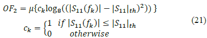
The objective function was eq. (21), where µ{…} represents the mean value of the argument and C k is a binary value that enables or disables the calculus of the k-th frequency component (f k ) in the design range. This function improves the performance of the antenna’s impedance matching through the minimization of the mean and standard deviation of the S 11 magnitude in the design range, and it adjusts the bandwidth to the established design.
The results obtained from the optimization processes are shown in Fig. 11, which presented a similar performance to the first antenna design (Section 4.1). The optimal objective function was -2.052 for the conventional PSO, while this value was -2.059 for PSOit. In both methods, the convergence criterion was to achieve the maximum number of iterations.

Source: Authors.
Figure 11 Objective function according to the iterations for the optimization of an UWB antenna with the PSO and PSOit.
Fig. 12 displays the S 11 magnitude as a function of frequency for the optimal antenna designs and the calculated initial design. It is observed that the calculated initial design does not cover the desired bandwidth and has a higher S 11 magnitude than the optimized ones. The optimal UWB antenna with the PSOit has a better performance considering the bandwidth adjustment to the established design (2 GHz), which was equal to 2.50 GHz, compared to the 2.60 GHz obtained with the conventional PSO. Both responses had a minimum resonant frequency of 1.50 GHz. Also, PSOit had a better result in the mean of the S 11 magnitude, which was equal to -22.45 dB in comparison with the PSO’s -22.14 dB.

4.3 Pixeled UWB antenna
The third antenna design consisted of a UWB PRMA with a pixeled resonant patch, i.e., the structure of the conductive patch is a matrix of 10x14 pixels, where each of them might be removed or present to improve the performance of the antenna. For the sake of simplicity, in this study, the pixels were designed with vertical symmetry, so they were ordered in an array of dimensions 10x7 and reflected. In this way, the optimization requires real and binary dimensions: the real dimensions were the separation between the lower edge of the resonating patch and the ground plane (p), the length and the wide of the radiant patch (L and W); and the binary dimensions were the presence of the 70 pixels (b 1, b 2 ,…, b 70), as it is shown in Fig. 13. When a pixel p is marked as present, b p =1. However, if the pixel should be removed, b p =0.

This design optimization required the application of the hybrid PSO (HPSO) and hybrid PSOit (HPSOit) to handle binary and real variables. The objective function, the calculated initial design, and the convergence criteria were those applied for the second design (Section 4.2).
When the resonant patch is simulated with the pixel matrix, there can be pixels that are connected only by the corner, leading to infinitesimal conductivity points between them. This was solved with the addition of an overlap equal to 0.1 mm in these cases to improve electrical conductivity [22].
In the optimization process, the first convergence criterion accomplished was that the value of particle did not change in a consecutive number of iterations. The HPSO finished the process in 154 iterations obtaining a minimum of -2.091, and the HPSOit did 144 iterations for a solution equal to -2.149, as shown in Fig. 14. Therefore, the performance of the optimization process was enhanced with the proposed method, thus obtaining a better response in a lower number of iterations.

Source: Authors.
Figure 14 Objective function according to the iterations for the optimization of a pixeled UWB antenna with the HPSO and HPSOit.
Regarding the performance of the optimal antenna, the adjustment of the bandwidth was equal to 2.50 GHz for both methods. The mean of the S 11 magnitude was -22.38 dB for the HPSO and -22.94 dB for the HPSOit, which represents an improvement (Fig. 15). Furthermore, the topologies of the optimal antennas are shown in Fig. 16, which had a few modifications between them.

Source: Authors.
Figure 15 Comparison of S 11 magnitude as a function of the frequency for the initial and optimized designs of the pixeled UWB antenna.

5. Conclusions
The main contribution of this article is the proposal of a PSOit modification and the presentation of its advantages for the optimal design of antennas. The proposed method was applied in the optimization process considering real and hybrid (real and binary) dimensions.
It was demonstrated that this method had a better performance in the typical benchmark functions than the conventional PSO. Likewise, the PSOit method had the best optimal response in the optimization of narrowband and UWB antenna designs, with an objective function based on the S 11 magnitude in the frequency range.
The modifications applied to the conventional PSO allow obtaining a better quality of solution than the conventional PSO, with the possibility of reducing the number of iterations to achieve the optimal result. Therefore, this method is a good alternative to be applied in antenna design optimization, which requires powerful methods to obtain the best results, given the complexity of the models.
Future work will be conducted in the application of the proposed method to PSO variants, which have been employed for the optimization of antennas or other electromagnetic devices, in order to evaluate their performance in the search for the best response in the same number of iterations or less.

