


 English (pdf)
 Article in xml format
 Article references
 Send this article by e-mail
 Cited by SciELO
  Cited by Google
  Similars in
SciELO
Similars in
SciELO  Similars in Google
 Permalink
1. Introduction
According to a report released by Mining and Energy Planning Unit (UPME, 2018), MMV Basin is a key tight oil and shale gas region, as shown in Fig. 1. This basin is located between the central and eastern mountain ranges of the Colombian territory. It is limited to the North with the Espiritu Santo fault system, to the North East with the Bucaramanga-Santa Marta fault system, to the South-East by the fault system Bituima and La Salina, to the South with the folded Girardot belt and to the West with the Neogene sediments that cover the Serranía de San Lucas and the basement of the Central Cordillera (Fig. 1).

The La Luna Formation is the principal Cretaceous source rock in the MMV basins. The integration of the lithological characteristics (type of rock, composition, thickness), the petroleum geochemistry parameters and an extensive production database have shown the considered lithological sequence, with excellent percentages of organic matter, higher than 2% TOC and thermally mature, constitutes hydrocarbon generators.
Physical characteristics of the rock type, such as its fractivity, lithological composition, silica content greater than 50%, continuous thicknesses greater than 100 feet, ensure greater operational success in the development of unconventional resources (Agencia Nacional de Hidrocarburos, 2012)(Martinez et al, 2011).
Given this promising data, the main objective of this study is to evaluate the technical and financial feasibility of exploiting this source rock reservoir. The study is original, due to the lack of literature on this type of study in a Colombian reservoir having these characteristics.
2.Methodology, materials and methods
2.1 Reservoir simulation
This study used the module of reservoir simulator of CMG to model multiple hydraulic fractures and simulate fluid flow behavior in tight oil reservoirs. A hydraulic fracture was modeled explicitly using local grid refinement (LGR), which captures the transient flow behavior from shale matrix to fracture (Rubin, 2010). Table 1 summarized the basic parameters required for the simulation. A basic reservoir model including multistage fractures is shown in Fig. 2.


Source: The authors
Figure 2 A basic reservoir model including 1 horizontal well and 23 hydraulic planar fractures.
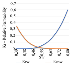
The assumed relative permeability curves, such a water-oil relative permeability and liquid gas relative permeability, are given in Fig. 3a and 3b, respectively. The base information is supported by the studies made by Ecopetrol (Empresa Colombiana de Petróleos), concluding that relative permeability curves in the Colombian shale formation are similar to some major oil-producing unconventional resource plays in North America. Actually, these properties compare favorably to the down dip and up dip trends for the Eagle Ford Formation (Cantisano, et al, 2013).


2.1.1 Sensitivity parameters
Seven uncertainty parameters were assessed, including fracture height, fracture half-length, fracture conductivity, hydraulic Fracture Spacing, Rock Compaction, Natural fracture aperture and Natural fracture conductivity. For each one, this study evaluated a reasonable range of values, with the actual maximum and minimum values based on public information of different reports (Cantisano, et al, 2013)(Benavides, 2017)(Ibañez et al, 2016), Table 2 includes the most relevant information extracted from the reports.
2.1.2 Model Assumption
The following assumptions were established for the evaluation of the model:
The reservoir is bounded by an upper and a lower impermeable layer.
The reservoir is isotropic and homogeneous with a constant height, porosity, and permeability.
The initial reservoir pressure is uniform.
The reservoir contains a slightly compressible fluid with constant oil density, viscosity, and compressibility.
Fluid flow takes place only through fractures.
There is no pressure loss along the wellbore.
No fracture hydraulic connection.
2.1.3 Grid
It was built a reservoir model with a volume of 7400ft X 3800ft X 310ft. The grid representing the reservoir has dimensions of de 94 X 49 X 10, where each cell has one volume de 80ft X 80ft X 31, common size of field blocks to capture a minimum number of frack- frack spacing. The hydraulic fractures are explicit represented by grid cells with a width of 2 ft, to reduce the number of blocks and the runtime, the fracture can be pseudoized to a width with this value. Number of refinement in I, J and K direction is 7 X 7 X 1.
2.1.4 Matrix subdivision
This study used a dual-permeability approach with logarithmic local grid refinement near fractures to increase numerical accuracy, while still maintaining computational efficiency. In the dual-permeability model, the porous medium was envisioned as two continuous: one significantly contributes to the pore volume but little to the flow capacity (matrix), while the other significantly contributes to the flow capacity with a negligible contribution to the pore volume (fracture). Yet, in the dual-permeability model, as the matrix continuum has non-zero permeability at the continuum level, the matrix-to-matrix fluid flow is still allowed to take place (Wijaya & Sheng, 2019). The governing equation for the oil-water dual-permeability model is given by:

u represents the phase fluxes, K is the absolute intrinsic permeability, K r is the relative permeability, μ is the dynamic viscosity, p is the phase pressure, ρ is the phase density and g is the gravity vector (Escobar et al, 2020).
2.1.5 Shape Factor
The shape factor describes the transmissibility between matrix and fracture. Kazemi and Gilman used the quasi-steady approximation, introduced by Warren and Root, and gave different formulas for the matrix shape factor (Kazemi, JR, & A.M, 1992) (Uribe et al, 2008), for a rectangle with all sides imbibing, the equation is given by:

F s is the shape factor; L x ,L y ,L Z is the natural fracture spacing in x, y and Z.; and V m is the volume matrix. Although the location of the fractures is not identified, there representation can be deduced from the shape factor.
2.1.6 Natural fracture porosity
Fracture porosity is required as input data to build the dual-permeability simulation model. It can be understood as the natural fracture width. Fracture porosity is estimated using the following expression:

It is worth highlighting that the fracture porosity is the porosity referenced to the Bulk Volume, not the porosity of the fracture area. The fracture porosity is really small, so no loss is register. In grid block bulk volume,
Thus,
Where DJ is the block width, DJFRAC is the natural of fracture space, DI is the direction and the length of the fracture, and DK is height. Similarly in j direction.
After replacing the (eq. 5) and (eq. 6) into the fracture porosity equation, the following equation is obtained:


When porosity fractures are rather small, some numerical difficulties can arise during the simulation run.

2.1.7 Natural permeability
Permeability defines the ability of porous medium to transmit fluids. The presence of open fractures has a great impact on the reservoir flow capacity. Therefore, the fracture permeability is an important factor that determines reservoir quality and productivity. The calculations for obtaining the natural fracture permeability are similar to those for obtaining the porosity, in particular the effective permeability.
Eqs. 8 and 9 show how the fracture permeability in i direction depends on the conductivity in the same direction and the number of fractures.

Or

Hence, basically, to obtain the fracture permeability, it is necessary to divide the intrinsic conductivity into the fracture space.
Regarding permeability in j direction, the calculations are the same as those for the i direction.
The permeability in the k direction is doubled only if the conductivity in the i direction is assumed to be the same as that of the j direction, as shown in the Eq. 10.

2.2. Economic evaluation
Integrating the reservoir model and the economic evaluation with a stochastic workflow helps to assess the unconventional opportunities. This study applied a staged approach using Monte Carlo simulation.
The customized tool provides a probabilistic framework for assessing oil projects regardless of their maturity. The focus was on capturing the key project components and their variability according to an intuitive workflow, and generating resource and economic metrics (Haskett & Brown, 2005). This facilitates a more rigorous comparison of opportunities and better decisions about where to drill the next wells. This also increases portfolio value and helps ensure capital expenditure focuses on projects that are likely to be commercial failures.
The financial analysis is developed through a probabilistic model using the software @Risk. The input and output data of the model cover a wide range via a probabilistic distribution. The economical calculations were adjusted to be performed prior income tax.
2.2.1. Inputs used for the financial Sensitivity Study
The incomes from the economic model depend on the outputs from the simulation, specifically the production forecasting.
The operational expenditures (OPEX) from the development stage of the well are mainly related to the production operational expenses, which include lifting costs, such as: flow-back water disposal, well maintenance, minor workover activities like reparations and general & administrative expenses. Transportation costs are also included in OPEX and include the transportation costs from the Valle Medio del Magdalena pipelines. Finally, the price discount of the Colombian blend relative to the dated Brent derived from this blend quality, being equal to 7% ECOPETROL REPORT, 2019. The value of the discount is an average from Valle Medio del Magdalena Basin discounts (Wood Mackenzie, 2020).
The average capital expenditures include capital associated with the drilling, completion, stimulation, and facilities. Due to the lack of references for forecasting input data in the economic analysis, since similar projects have never been developed in Colombia, this study used as benchmark the investments and costs in the most important reservoirs in the United States (U.S. Energy Information Administration, 2016), Canada (Mistré, 2017), and Argentina (Rassenfoss, 2018). Table 3 summarized the inputs for the financial analysis.

2.2.2. Economic metrics
Net Present Value and Internal rate of return are the most common metrics to evaluate the economic viability of a project - see Eqs. 11 and 12 (Brealey & Myers, 2014)

NPV is net present value, CF is the cash flow after-tax, r 1 is the discount rate and T is cash flow time

IRR is the Internal rate of return, CF cash flow after-tax, r 1 is the discount rate, T is cash flow time and CF 0 is the total initial investment. To evaluate the project was taken into account these criteria.
For a single project be successful, its NPV should be positive.
For independent projects: successful if their IRR are greater than some fixed IRR, the threshold rate/hurdle rate.
Colombia's oil fiscal regime is regressive. The government captures a lower profit share from more valuable fields and a higher profit share from less valuable fields.
Similarly, in Colombia, an average tax of 6% of the lifting cost of the oil produced is generated, which may increase depending on the value of the basin produced. At present there is no legislation in force referring the oil from unconventional reservoirs. Therefore, this work assumes the national average value already in course in the country for conventional reservoirs.
3.Results and discussions
3.1. Model results
The model was run for the initial parameters of the reservoir; including an Oil & Water contact at 10105 ft and a reference pressure of 8068 psi at 9840 ft. Fig. 4 shows the changes of the pressure after five years of production. The run time of is 30 years.

Source: The authors
Figure 4 A basic reservoir model including 1 horizontal well and 23 hydraulic planar fractures.
After performing numerical simulations for the case study, the rate of oil production and cumulative oil production were obtained - see Fig. 5 and Fig. 6, respectively. Findings show that there is a wide range of oil rate and cumulative oil production. The ranges for oil rate and cumulative oil production at a 30-year period are obtained as 1.18-1.46 MMBL, which corresponds to a daily production of 35 - 39 bld respectively. The average cumulative oil production and the oil rate were 1.21 MMBL which corresponds to a daily production of 36.9 bld respectively. It is important to note that the oil rate curve in tight oil declines in a short time.


The reservoirs containing light oils have more dissolved gases than reservoir with heavy oils. Therefore, it would be interesting to determine the GOR ranges obtained in the model. The ranges for Solution Gas-Oil Ratio are obtained as 540-573 ft3/bbl, the average was 555 ft3/bbl, as show in Fig. 7.

The findings are, then, used to build the half-normal plot and the Tornado Diagram to identify the ranking of significant factors affecting cumulative oil production. The half-normal plot at different periods of production for cumulative oil production are presented in Fig. 8. Any parameter or two-parameters interaction highly deviating from the straight line are recognized as the factors that affect the oil production significantly.

The significant and insignificant model parameters are determined by the Tornado Diagram - see Fig. 9. The rank of important parameters can provide critical insights into performing history matching with field production data in a short-term period. The main influence parameters are the fracture spacing and the fracture half-length.

3.2. Economic results
Based on the production profiles and the assumed expenditures, blend discount-price and fiscal regime, the cash flow model was applied for three scenarios (minimum, mean and maximum) - see Fig. 10.

Results from the economic evaluation are shown in Figs. 11 and 12. The success probability is 27.5% (NPV≥ 0), and 27.7% (>Discount Rate of 10% p.y), depending on the metric used.

For the Colombian hydrocarbon sector, the valuation of projects usually applies a real discount rate of 10% p.y., as the minimum profitability that the shareholders expect to obtain. For instance, by considering the reports of the main operating companies with contracts with the National Agency of Hydrocarbons to develop activities in Unconventional Reservoirs, and performing an analysis based on the companies´ financial statements, the range of return found hovers between 10%-12% p.y.(CREG, 2014). This includes the national territory in exploratory Blocks located in the Magdalena basins (Parex Resources Colombia Ltd. Conoco Phillips, Canacol Energy Ecopetrol and Exxon Mobil).
The parameters with high uncertainty are identified by analyzing the Tornado Diagram. The Brent Price and production are the most critical parameters for the NPV, with a positively impact on the project. On the other hand, Fig. 12 shows how completion and lifting cost parameters negatively affects the project.


The IRR tornado diagram is analyzed in the same way. While completion and lifting cost are the pivotal parameters for the IRR, negatively affecting the project, Brent price and production parameter positively affects the project.
4.Conclusions
Through numerical simulations of the rate of oil production and cumulative oil production, there is a wide range of oil rate and cumulative oil production in the assessed basin. The ranges for oil rate and cumulative oil production at 30 years were 1.18-1.46 MMBL, (daily production of 35 - 39 bld respectively), and the average cumulative oil production and the oil rate were 1.21 MMBL (daily production of 36.9 bld respectively). The ranges for Solution Gas-Oil Ratio were 540-573 ft3/bbl, the average was 555 ft3/bbl.
According to financial results, the success probability is 27.5% (NPV≥ 0), and 27.7% (>Discount Rate of 10% annual) is the success probability from an IRR analysis.
The completion and lifting cost are the pivotal parameters for the IRR negatively affecting the project, BRENT price and production parameter positively affect the project.

