Introduction

Dystocia in cattle results in many adverse consequences for the dam and its offspring (^{Azizzadeh et al., 2012}; ^{Barrier et al., 2012}). These include increased calf morbidity and mortality, decreased fertility and milk production, low cow survival and reduced welfare (^{Mee et al., 2011}). There are also many direct and indirect factors affecting the incidence of dystocia in cattle. The first group comprises feto-pelvic disproportion, fetal malposition, vulvar or cervical stenosis, and uterine torsion, whereas the second group includes dam’s age at calving, gestation length, parity, body weight, and condition at service and calving, calf sex, sire, breed and strain, feeding, and climate, etc. (Mee, 2008). In order to prevent the occurrence of dystocia and alleviate its negative effects, it would be desirable to develop prognostic methods capable of indicating animals with potential problems at calving, based on the above-mentione risk factors. One such approach involves the use of statistical methods, especially those from the field of data mining. There are numerous data mining algorithms, some of which have already been applied to animal farming (^{Piwczyński et al., 2013}). Decision trees, belonging to this group of algorithms, are characterized by a relatively easy interpretation and implementation. However, each type of algorithm has some unique features which make it better or worse suited for certain tasks. Thus, it is advisable to compare the effectiveness of several such methods in solving a given problem.

Therefore, the first aim of our study was to classify calving difficulty in dairy heifers using three different types of decision trees [classification and regression trees (CART), chi-square automatic interaction detection trees (CHAID), and quick, unbiased, efficient, statistical trees (QUEST)], and to compare the results of this classification with those of a more traditional statistical method (i.e. a generalized linear model; GLM). The second aim was to identify the most significant factors affecting calving course.

Materials and methods

Model construction and evaluation

Of the numerous data mining algorithms, decision trees are characterized by a relatively fast construction process and easy interpretation of a final model (^{Witten et al., 2011}). They are based on a “divide-and-conquer” approach to the problem of learning from a set of independent observations (cases). Individual nodes within the tree test particular attributes (predictors

Table 1 Means and standard deviations of continuous independent variables. 

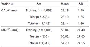
1Calving age. 2Sire’s rank based on the mean calving difficulty scores of its daughters (without units). SD: Standard deviation

Table 2 Distributions of categorical variables. 

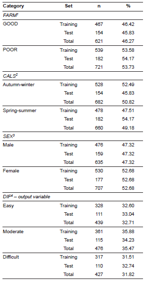
1Category of the farm where the heifer was kept based on its average milk yield (POOR: <10,200 Kg, GOOD: ≥ 10,200 Kg). 2Calving season. 3Calf sex. 4Calving difficulty

or independent variables), whereas terminal nodes (called “leaves”) indicate the class to which each observation reaching this node belongs (^{Witten et al., 2011}). In our study, three different types of decision trees [classification and regression trees (CART), chi- square automatic interaction detection (CHAID), and quick, unbiased, efficient, statistical trees (QUEST)] were applied. The CART algorithm builds binary trees (with each parent node split into two child nodes) by the iterative checking of all possible values of the independent variables (predictors) in order to identify the one on which the split in a parent node will be based (the so-called splitter) as well as the cut-off point for the split so that the resulting child nodes contain the groups of cases as homogeneous as possible (^{Speybroeck, 2011}). The process is repeated until it is no longer possible to make additional splits, but the tree obtained in this way is frequently too complex and overfit to the training data and must be reduced in the so-called “pruning” step (^{Moisen, 2008}). In the case of CHAID, the splits are not limited to binary ones and the chi-square test is used to determine the best split at each stage of tree growing. Moreover, CHAID stops adding new nodes before overfitting occurs and makes direct use of only categorical independent variables so continuous (numerical) variables are first discretized into separate intervals (^{Chang, 2007}). Finally, QUEST generates binary trees by merging classes into two groups before splitting and using quadratic discriminant analysis to determine the best split. As a result, two potential splitting points are obtained, from which the one closer to the mean value of the analyzed variable in a population of vectors belonging to one of the clusters is selected (^{Loh and Shih, 1997}).

In the development of CART, equal costs of misclassification and the Gini index as a measure of node impurity were used. The a priori probability of class membership was estimated from the training sample. The stop criterion was the minimization of misclassification error with a minimal node size of 134 cases. Moreover, 10-fold cross-validation was used to find the best tree structure understood as a compromise between the tree complexity and its quality. In the construction of the CHAID trees, a modification of the standard algorithm was applied (i.e. exhaustive CHAID), which conducts a more thorough search for the predictor that yields the most significant split (i.e. the merging of predictor categories is carried out until only two categories remain; ^{Hill and Lewicki, 2006}). When growing the exhaustive CHAID tree, the misclassification costs and the minimal tree node size were like in the CART analysis, whereas the p-value for splitting was equal to 0.05. Moreover, the Bonferroni adjustment and the 10-fold cross validation were applied to find the best model. The parameters for the last analyzed tree algorithm (QUEST) included: The apriori probability estimated from the training sample, equal costs of misclassification, minimization of misclassification error as a stop criterion (minimal leaf size equal to 5, standard error rule equal to 1.0), the 10-fold cross-validation, and the p-value for split variable selection equal to 0.05.

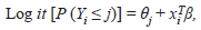
Finally, the GLM model with an ordinal multinomial distribution for the dependent variable (calving difficulty score) and a logit link function was applied according to the following formula:

Where:

^_Yi = is the ith observation of the dependent variable (calving difficulty score).

j = is the calving category (easy, moderate, or difficult).

^_θj = is the intercept for the ^_jth category.

^_xi = is a vector of explanatory variables for the _^ith

observation.

β = is the corresponding set of regression parameters.

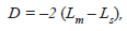
To assess the goodness of fit of GLM, the deviance statistic (D) was calculated:

Where:

^_Lm = is the maximized log-likelihood for a given model.

^_Ls = is the log-likelihood for the saturated model (i.e. the most complex model for the selected distribution of the dependent variable and a link function).

The assumptions of GLM were also tested (i.e. the normal distribution of residuals, the lack of predictor collinearity, and outliers).

After growing the trees and estimating the GLM parameters, their classification quality was evaluated on the L set. The proportions of correctly classified calvings from each of the three distinguished categories (easy, moderate, and difficult) as well as overall accuracy (the proportion of correctly classified cases from all classes) were calculated and the differences in these proportions were tested for statistical significance using the McNemar test for dependent samples with the Bonferroni correction for multiple comparisons. Statistical significance was set at p ≤ 0.05. Moreover, all types of models were verified on the independent T set to evaluate their ability to correctly predict calving difficulty class during their potential practical application. The proportions of correct classifications on the T set were again compared with the test for proportions. It should be added that the learning (or training) set (L) was used to build and train the tree models and to estimate the GLM parameters, whereas the test set (T) comprising new data (calvings), not seen previously by the models during their development, was used to verify their predictive capabilities. This results from the fact that the post hoc prediction is almost always too optimistic since the models are verified on the same data that were used for their construction. Consequently, a new data subset (the test set) separated from the whole dataset of records is necessary to objectively assess the a priori predictive performance of the model.

To complement the analysis of model performance, the cumulative gains charts were also plotted (based on the test set) to show the relationship between the gains (defined as a proportion of correctly classified cases out of all the cases in the population belonging to a given category) and the considered sample size for the three types of classification trees and GLM (^{Nisbet et al., 2009}). Model construction and evaluation was performed using Statistica 10 software (StatSoft Inc., Tulsa, OK, USA).

Results

Discussion

In the case of the CART and CHAID trees, the first split was based on either the SIRE or FARM variable. The SIRE was also used for the first split in the QUEST tree (Figures 1-3).

In the study by ^{Piwczyński et al. (2013}) on the use of CART and CHAID for the analysis of significant predictors of calving difficulty in Polish Holstein- Friesian black-and-white cows, the first division of the whole data set in the root node was based on lactation number. The two subsequent divisions were based on calf birth weight and the third one on pregnancy length and this variable was used for splitting twice (at the threshold values of 282 and 284 days, respectively). In the above-mentioned study, the last considered splitting variable was management system. It should be noted that although the CART and CHAID trees in our study and that by Piwczyński et al. (2013) utilized a similar set of independent variables, the final structure of the resulting decision trees was somewhat different. Obviously, some factors described by Piwczyński et al. (2013; such as lactation number) were not available in our study, which included only heifers.

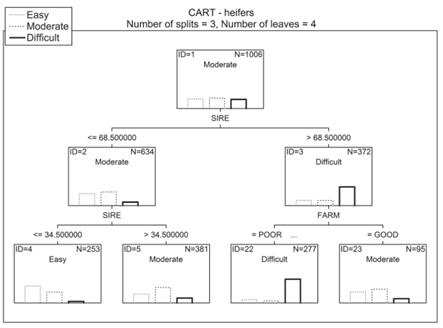
Figure 1 Classification and regression tree (CART) model for the classification of calving. SIRE: Sire’s rank based on the mean calving difficulty scores of its daughters. FARM: Category of the farm where the animal was kept based on its mean milk yield (POOR: <10,200 Kg, GOOD: ≥ 10,200 Kg). Node labels are assigned according to the most numerous category. 

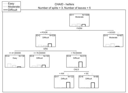
Figure 2 Chi-square automatic interaction detection (CHAID) model for the classification of calving. SIRE: Sire’s rank based on the mean calving difficulty scores of its daughters. FARM: Category of the farm where the animal was kept based on its mean milk yield (POOR: <10,200 Kg, GOOD: ≥ 10,200 Kg). CALS: Calving season (AW - autumn-winter, SS - spring-summer). Node labels are assigned according to the most numerous category. 

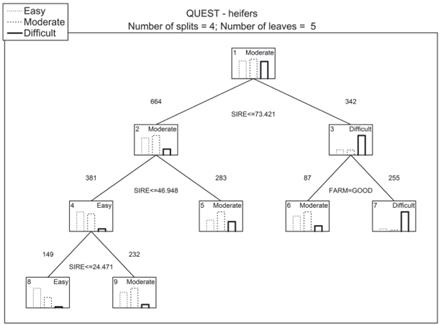
Figure 3 Quick, unbiased, efficient, statistical trees (QUEST) model for the classification of calving (cases satisfying the splitting condition in a parent node go to its left child node). SIRE: Sire’s rank based on the mean calving difficulty scores of its daughters. FARM: Category of the farm where the animal was kept based on its mean milk yield (POOR: <10,200 Kg, GOOD: ≥ 10,200 Kg). Node labels are assigned according to the most numerous category. 

Table 3 Estimated parameters of the generalized linear model (GLM). 

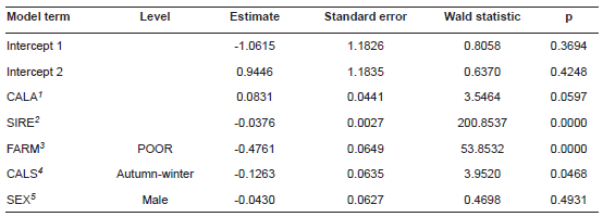
1 Calving age. 2 Sire’s rank based on the mean calving difficulty scores of its daughters. 3 Category of the farm where the animal was kept based on its mean milk yield (POOR: <10,200 Kg, GOOD: ≥ 10,200 Kg). 4 Calving season. 5 Calf sex. Variables with p-values less than 0.05 are marked in bold

In the case of GLM, the value of the applied goodness-of-fit criterion (i.e. the deviance statistic relative to its degrees of freedom; 0.92) testified to the good overall quality of the constructed GLM model as the values of approximately 1.0 are considered to show a good fit of the model to the training data (McCullagh and Nelder, 1989). However, since not all the assumptions of the GLM model (in principle required) were met, its application in some situations may not be fully recommended from a purely statistical point of view.

Table 4 Proportions of correctly classified calvings on the training and test sets. 

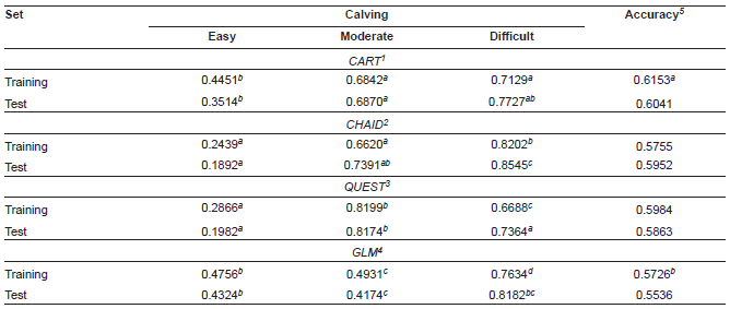
a-d Values marked with different superscript letters within a column (and a set) differ significantly (p ≤ 0.05). 1 Classification and regression trees. 2 Chi-square automatic interaction detection. 3 Quick, unbiased, efficient, statistical trees. 4 Generalized linear model. 5 Accuracy: Proportion of correctly classified cases from all classes.

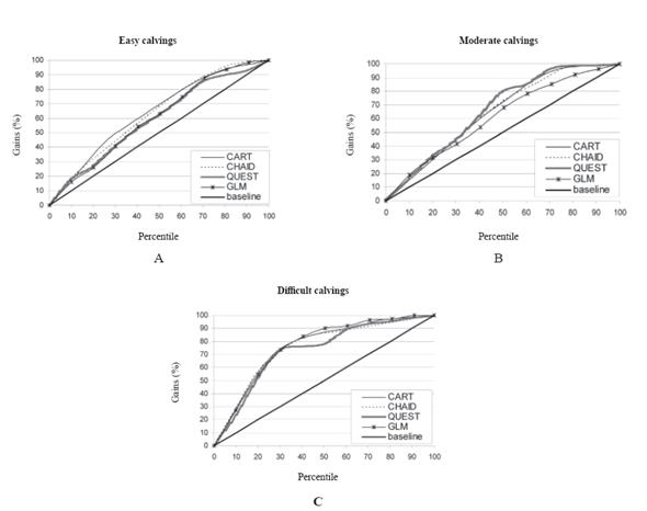
Figure 4 Gains chart for individual calving categories: A= easy, B = moderate, C = difficult. CART: Classification and regression trees. CHAID: Chi-square automatic interaction detection. QUEST: Quick, unbiased, efficient, statistical trees. GLM: Generalized linear model. 

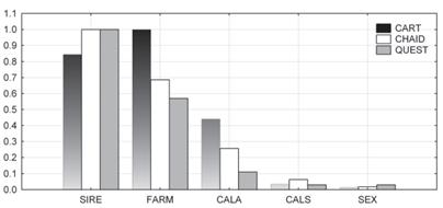
Figure 5 The importance of individual predictors of calving difficulty for the tree models. SIRE: Sire’s rank based on the mean calving difficulty scores of its daughters. FARM: Category of the farm based on its mean milk yield. CALA: Calving age. CALS: Calving season. SEX: Calf sex. CART: Classification and regression trees. CHAID: Chi-square automatic interaction detection. QUEST: Quick, unbiased, efficient, statistical trees. 

As far as the model quality evaluated on the L set is concerned, CART and GLM were most effective in classifying easy calvings (44.51 and 47.56% correctly indicated easy cases, respectively), whereas QUEST was most efficient in predicting moderate calvings (81.99%). The CART and CHAID were also quite effective in this respect (68.42 and 66.20%, respectively) compared with GLM, for which the proportion of correctly indicated moderate cases was the lowest (49.31%). The greatest number of difficult calvings was properly classified by CHAID and GLM (82.02 and 76.34%, respectively), while the diagnosis made by CART and QUEST was significantly less accurate (71.29 and 66.88%, respectively). In this context, CHAID and GLM would be preferable under conditions in which the highest dystocia detection rate is the priority. However, GLM was also able to properly indicate most easy calvings, which is advantageous from the farmer’s point of view, since the number of false alarms generated by the model would be the lowest in this case.

In general, the accuracy obtained on the L set for the three distinguished categories of calving course (approximately 60%) in our study was moderate (Table 4). It was similar to that (61.50%) reported by ^{Piwczyński et al. (2013}), who established four different categories of calving difficulty. It was also comparable to the accuracy (50 to 60.20%) recorded by ^{Johnson et al. (1988}), who studied the possibility of dystocia detection (with the five classes of calving difficulty) in Hereford heifers using discriminant function analysis. The accuracy reported by the aforementioned authors depended on the set of predictors included in the forecasting model and increased to approximately 85.50% with only two classes of calving ease. With the same number of distinguished delivery classes (dystocia vs eutocia), ^{Arthur et al. (2000}) obtained very similar accuracy (85.20 to 91.70%) using the same method as above for dystocia diagnosis in Angus heifers. This value was much higher than that in our study (Table 4), where the three classes of calving difficulty were considered. This comparison between different model types shows that the final classification accuracy depends to some extent on the number of categories of the dependent variable. The division into only two classes usually yields better results in terms of the number of correct classifications, but such a model loses some information on the possible calving course. Taking into account the real number of calving difficulty categories distinguished by the official recording scheme in our country (which is six at present), an attempt was made in our study to more accurately indicate calving class.

After evaluating model quality, the predictive performance of individual decision trees and GLM was objectively verified on the independent T set, which was not used during the tree growing and GLM estimation stage and which could show the real ability of the models to properly predict calving categories during their potential practical application. The results obtained earlier on the L set were generally confirmed on the T set. And so, GLM and CART were most accurate in predicting easy calvings (43.24 and 35.14%, respectively), whereas CHAID and QUEST were the most effective classifiers for the moderate calvings (73.91 and 81.74%, respectively). The lowest ability to correctly indicate moderate calvings was exhibited by GLM (41.74%). The highest proportion of difficult cases was properly diagnosed by CHAID and GLM (85.45 and 81.82%, respectively), whereas CART and QUEST were significantly less successful in classifying this type of calvings (77.27 and 73.64%, respectively). In general, the accuracy on the T set in our study was moderate (Table 4), and it was approximately 10 to 30% lower than the values (72.60 to 90.30%) reported by ^{Arthur et al. (2000}), who investigated dystocia detection in Angus heifers. However, the better results presented by Arthur et al. (2000) can partially be attributed to the lower number of calving classes. Moreover, although the prediction models based on discriminant function analysis could accurately predict normal calvings (specificity in the range of 72.60 to 90.30%), their ability to properly predict dystocia in Angus heifers was much lower (sensitivity ranging from 0 to 40.00%). Finally, it was not possible to compare the results obtained on the independent test set in our study with those of ^{Piwczyński et al. (2013}) and ^{Johnson et al. (1988}) because they did not report the outcomes of the validation procedure.

On the other hand, a high proportion of correct classifications of dystocia cases (the difficult class) in the heifer T data set (73.64 to 85.45%) in our study is especially noteworthy. This may make it possible for a farmer or herd manager to undertake appropriate measures in order to prevent adverse consequences of dystocia in a heifer. It is also important to consider that models with high sensitivity would be preferred under field conditions as the misclassification of an easy calving by the model is not so costly (additional labor associated with cow watching) as the misdiagnosis in the opposite direction (missing a dystocia case). However, it is also desired for the model to have possibly high specificity, as a large number of false alarms are troublesome for the farmer and decrease his trust in the system. We would also like to emphasize that the percentage of correctly diagnosed moderate calvings (i.e. those requiring help from man or the use of mechanical equipment) by decision trees in our study was relatively high (68.70 to 81.74%). In this respect, data mining models in the form of classification trees turned out to be superior to GLM, for which this proportion was the lowest (41.74%).

Finally, the shape of the curves plotted on the cumulative gains charts revealed the relatively good performance of all the classifiers investigated (Figure 4). The closer the curve approaches the upper left corner of the graph [the (0, 1) point], the better the discriminative power of the model is. As can be seen in Figure 4, QUEST and GLM were characterized by slightly lower gains than CART and CHAID for easy calvings, but QUEST generated somewhat higher gains for moderate deliveries, for which GLM presented the worst results. However, the gains produced by all the classifiers were greatest for the difficult category. Of the data mining models (three different types of decision trees) used in our study, the best predictive performance was in general characteristic of CHAID, although it should be emphasized that there were not any significant differences in the accuracy on the T set. Nevertheless, CHAID exhibited the highest proportion of correctly predicted difficult calvings (dystocia) in heifers at a relatively large number of properly diagnosed moderate deliveries. Only its ability to accurately indicate easy calvings was lower (only approximately one-fifth of all cases), which needs to be considered by the farmer if such a model is implemented in a farm.

The comparison of the data mining algorithms with a more traditional statistical method (i.e. the GLM model, used as a reference in our study) showed that both types of classifiers yielded comparable results. Somewhat larger differences were found for the easy and moderate category, but the overall accuracy was also very similar. Therefore, it is not possible to explicitly confirm the superiority of data mining models (in the form of decision trees) over more traditional statistical techniques (GLM in this case) based on the prediction results of our study. However, parametric methods such as GLM require the fulfillment of various assumptions, from which not all were met in our study. Moreover, the structure of the classification trees is more easily interpretable (even by non-experts) than the coefficients of the GLM model, which facilitates the understanding of the investigated relationships between different factors and calving course.

The second stage of our study was the identification of the most influential factors affecting calving difficulty. The most important predictor for all the three decision tree types was SIRE. Also, CALA and FARM were found to considerably affect the category of calving difficulty. In the case of GLM, the only significant effects were SIRE, FARM, and CALS.

The rank of the dam’s sire was based on the mean calving difficulty score of its daughters. The goal of including this predictor in the tree models and GLM was to take into account the genetic component of dystocia represented by the dam’s sire effect. Although, it is not possible to directly include a sire effect in the prediction model, it can be incorporated into it in a more general form (e.g. a rank), which orders sires according to the calving difficulty level experienced by their daughters. In a recent study by ^{Mee et al. (2011}), it was found that the relationship between predicted transmitting ability for maternal calving difficulty and the probability of assisted parturition depended on dam parity and calf sex. It was stronger for lower parities and male sex calves.

The next important factor was the category of the farm where the heifer was kept (FARM; Figure 5). As can be seen from Figures 1-3, the POOR category was associated with a markedly higher number of difficult calvings. This relationship could have resulted from the worse husbandry conditions on the farm, including poorer control of difficult calvings. However, this result is not entirely consistent with that reported by ^{Gröhn et al. (1990}), who investigated different factors affecting reproductive disorders in Finnish Ayrshires, and found that higher herd milk yield in the current lactation was associated with an increased risk of dystocia. On the other hand, the only herd-level factor included in the analysis of dystocia incidence in Irish Holstein-Friesians (^{Mee et al., 2011}; i.e. herd size), did not significantly affect the frequency of difficult parturitions.

The last important predictor for decision trees was calving age (CALA; Figure 5). The greatest difference in dystocia occurrence is found between heifers and cows (^{Norman et al., 2010}; ^{Atashi et al., 2012}). Generally speaking, the optimal age at first calving in dairy heifers is 22 to 24 months (^{Ghavi Hossein-Zadeh, 2013}), although a recent study on seasonally calving Holstein-Friesian heifers (^{Berry and Cromie, 2009}) suggested that this age should be 25 to 27 months with respect to calving ease. In the cited study, heifers calving at the age of 22 months had a higher risk of calving assistance than those calving at 24 months of age, whereas heifers calving at 25 to 27 and 35 months of age had a lower risk of such assistance compared with the animals calving at 24 months of age. Also, body weight at breeding or calving may affect calving difficulty. It can be even a better predictor of dystocia than age at first calving itself, but it is much more difficult to be consistently recorded. As a result of greater growth rates, heifers currently calve for the first time relatively earlier but with a high body weight. Consequently, calvings in such heifers are usually easier compared with those of their lighter herdmates. Finally, it should be emphasized that some authors (^{Hickey et al., 2007}; ^{Bazzi, 2010}; ^{Yıldız et al., 2011}) did not confirm any significant relationship between calving age and difficulty.

The other significant predictor of calving difficulty identified by the GLM model was also calving season (CALS). It is generally considered that under European climatic conditions, calvings occurring in autumn and winter tend to be more difficult than those in the spring-summer season, which may result from increased gestation length, calf birth weight, and stillbirth rate in the colder season and less intensive supervision of calvings and more physical exercises in summer (^{Mee et al., 2011}).

In conclusion, the tree classification models obtained in our study showed promise in predicting individual classes of calving difficulty in dairy heifers; however, their further improvement would be necessary to obtain better accuracy. The most influential factors affecting difficulty level included: The rank of the dam’s sire, calving age, and the yield category of a farm and calving season. Our study showed that decision trees (after improvement of their predictive performance) could be potentially applied as an accessory tool to aid farmer in making decisions concerning calving management, especially considering that the created rules are relatively simple and easily interpretable.

Acknowledgements

This work was supported by the Polish Ministry of Science and Higher Education (grant number 517- 01-028-3962/17).

Conflict of interest

The authors declare they have no conflicts of interest with regard to the work presented in this report