


 English (pdf)
 Article in xml format
 Article references
 Send this article by e-mail
 Cited by SciELO
  Cited by Google
  Similars in
SciELO
Similars in
SciELO  Similars in Google
 Permalink
1. Introduction
Let (Ω, A, ν) be a measurable space consisting of a set Ω, a σ-algebra A of subsets of Ω and a countably additive and positive measure ν on A with values in [0, +∞] . For a ν-measurable function w : Ω →  , with w (x) ≥ 0 for ν-a.e. (almost every) x ∈ Ω, consider the Lebesgue space

For simplicity of notation we write everywhere in the sequel  wdν instead of
  w (x) dν (x). Assume also that
  wdν = 1.
We say that the pair of measurable functions (f, g) are synchronous on Ω if
 (1)
(1)
for ν-a.e. x, y ∈ Ω. If the inequality reverses in (1), the functions are called asynchronous on Ω.
If (f, g) are synchronous on Ω and f, g, fg ∈ Lw (Ω, ν), then the following inequality, that is known in the literature as Chebyshev’s Inequality, holds:
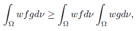 (2)
(2)
where w (x) ≥ 0 for ν-a.e. (almost every) x ∈ Ω and  wdν = 1.
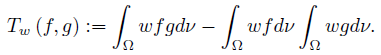
If f, g : Ω →  are ν-measurable functions and f, g, fg ∈ Lw(Ω, ν), then we may consider the Chebyshev functional
The following result is known in the literature as the Grüss inequality:
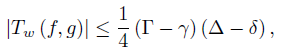 (3)
(3)
provided
 (4)
(4)
for ν-a.e. x ∈ Ω.
The constant  is sharp in the sense that it cannot be replaced by a smaller quantity.
If f ∈ Lw (Ω, ν), then we may define
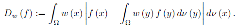 (5)
(5)
The following refinement of Grüss inequality in the general setting of measure spaces is due to Cerone & Dragomir [1]:
Theorem 1.1. Let w, f, g: Ω →  be ν-measurable functions with w ≥ 0 ν-a.e. on Ω and
 wdν = 1. If f, g, fg ∈ Lw (Ω, ν) and there exist constants δ, ∆ such that
 (6)
(6)
then we have the inequality
 (7)
(7)
The constant is sharp in the sense that it cannot be replaced by a smaller quantity.
Motivated by the above results, we introduce in this paper the concept of quadruple D−synchronous functions that generalizes the concept of a pair of synchronous functions, we establish an inequality similar to Chebyshev inequality and also provide some CauchyBunyakovsky-Schwarz type inequalities for a functional associated with this quadruple. Some applications for univariate functions of real variable are given. Discrete inequalities are also stated.
2. D−Synchronous functions
Let (Ω, A, ν) be a measurable space and f, g, h, ℓ : Ω →  be four ν-measurable functions on Ω.
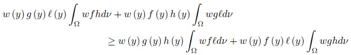
Definition 2.1. The quadruple (f, g, h, ℓ) is called D−Synchronous (D−Asynchronous) on Ω if
 (8)
(8)
for ν-a.e. (almost every) x, y ∈ Ω.
This concept is a generalization of synchronous functions, since for g = 1, ℓ = 1 the quadruple (f, g, h, ℓ) is D−Synchronous if, and only if, (f, h) is synchronous on Ω.
If g, ℓ 0 ν-a.e on Ω, then
 (9)
(9)
for ν-a.e. x, y ∈ Ω. So, if gℓ > 0 ν-a.e on Ω the quadruple (f, g, h, ℓ) is D−Synchronous if, and only if,  is synchronous on Ω.
Theorem 2.2. Let f, g, h, ℓ: Ω →  be ν-measurable functions on Ω and such that the quadruple (f, g, h, ℓ) is D-Synchronous (D−Asynchronous), w ≥ 0 a.e. on Ω with
 wdν = 1 and fh, gℓ, gh, f ℓ ∈ Lw
(Ω, ν). Then,
wdν = 1 and fh, gℓ, gh, f ℓ ∈ Lw
(Ω, ν). Then,
 (10)
(10)
Proof. Since the quadruple (f, g, h, ℓ) is D−Synchronous, then
 (11)
(11)
for ν-a.e. x, y ∈ Ω.
This is equivalent to
 (12)
(12)
for ν-a.e. x, y ∈ Ω.
Multiply (12) by w (x) w (y) ≥ 0 to get
 (13)
(13)
for ν-a.e. x, y ∈ Ω.
If we integrate the inequality (13) over x ∈ Ω, then we get
 (14)
(14)
for ν-a.e. y ∈ Ω.
Finally, if we integrate the inequality (14) over y ∈ Ω, then we get

which is equivalent to the desired result (10).
Corollary 2.3. Let f, g, h, ℓ: Ω →  be ν-measurable functions on Ω and such that gℓ > 0 ν-a.e on Ω,
  is synchronous (asynchronous) on Ω, w ≥ 0 a.e. on Ω with
 wdν = 1 and fh, gℓ, gh, fℓ ∈ Lw (Ω, ν) ; then the inequality (10) is valid.
Let f, g, h, ℓ : Ω →  be ν-measurable functions on Ω , w ≥ 0 a.e. on Ω with
  wdν = 1 and fh, gℓ, gh, fℓ ∈ Lw (Ω, ν) ; then we can consider the functionals
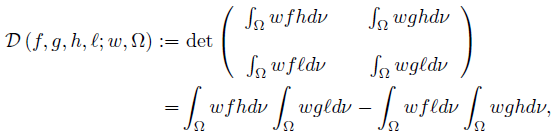 (15)
(15)
and, for (f, g) = (h, ℓ),
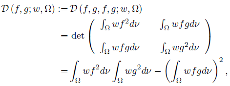 (16)
(16)
provided f 2, g2 ∈ Lw (Ω, ν).
We can improve the inequality (10) as follows:
Theorem 2.4. Let f, g, h, ℓ: Ω →  be ν-measurable functions on Ω and such that the quadruple (f, g, h, ℓ) is D−Synchronous, w ≥ 0 a.e. on Ω with
 wdν = 1 and fh, gℓ, gh, fℓ ∈ Lw (Ω, ν) ; then,
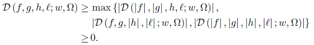 (17)
(17)
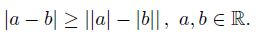
Proof. We use the continuity property of the modulus, namely
Since (f, g, h, ℓ) is D−Synchronous, then
 (18)
(18)
for ν-a.e. x, y ∈ Ω.
As in the proof of Theorem 2.2, we have the identity
 (19)
(19)
By using the identity (19) and the first branch in (18) we have

which proves the first part of (17).
The second and third part of (17) can be proved in a similar way and details are omitted.
3. Further results for the functional D
We have the following Schwarz’s type inequality for the functional D:
Theorem 3.1. Let f, g, h, ℓ: Ω →  be ν-measurable functions on Ω , w ≥ 0 a.e. on Ω with
 wdν = 1 and f2, g2, h2, ℓ2 ∈ Lw (Ω, ν). Then,
 (20)
(20)
Proof. As in the proof of Theorem 2.4, we have the identities


and

By the Cauchy-Bunyakovsky-Schwarz double integral inequality we have
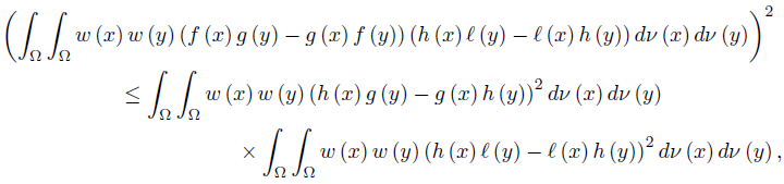
which produces the desired result (20).
Corollary 3.2. Let f, g, h, ℓ: Ω →  be ν-measurable functions on Ω with g2, ℓ2 ∈ Lw (Ω, ν), w ≥ 0 a.e. on Ω with
 wdν = 1, and a, A, b, B ∈
  such that A > a, B > b,
 (21)
(21)
ν-a.e. on Ω. Then,
 (22)
(22)
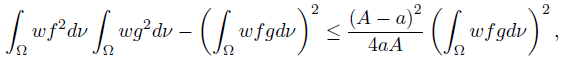
Proof. In [2] (see also [4, p. 8]) we proved the following reverse of Cauchy-BunyakovskySchwarz integral inequality

provided that ag ≤ f ≤ Ag ν-a.e. on Ω and g2 ∈ Lw (Ω, ν).
Since, we also have

provided that bℓ ≤ h ≤ Bℓ ν-a.e. on Ω and ℓ2 ∈ Lw (Ω, ν). Then, by (20) we have

that is equivalent to the desired result (22).
For positive margins we also have:
Corollary 3.3. Let f, g, h, ℓ: Ω →  be four ν-measurable functions on Ω with g2, ℓ2 ∈ Lw (Ω, ν), w ≥ 0 a.e. on Ω with
 wdν = 1, and a, A, b, B > 0 such that A > a, B > b,
 (23)
(23)
ν-a.e. on Ω. Then we have
 (24)
(24)
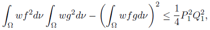
Proof. In [3] (see also [4, p. 16]) we proved the following reverse of Cauchy-BunyakovskySchwarz integral inequality:
whenever ag ≤ f ≤ Ag ν-a.e. on Ω.
Since

provided bℓ ≤ h ≤ Bℓ ν-a.e. on Ω, then by (20) we get the desired result (24).
If bounds for the sum and difference are available, then we have:
Corollary 3.4. Let f, g, h, ℓ : Ω →  be ν-measurable functions on Ω with g2 , ℓ2 ∈ Lw (Ω, ν), w ≥ 0 a.e. on Ω with
 wdν = 1. Assume that there exists the constants P1, Q1, P2, Q2such that
 (25)
(25)
a.e. on Ω; then,
 (26)
(26)
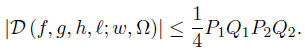
Proof. In the recent paper [5] we obtained amongst other the following reverse of CauchyBunyakovsky-Schwarz integral inequality:
provided |g − f| ≤ P1, |g + f| ≤ Q1 a.e. on Ω.
Since

if |h − ℓ| ≤ P2, |h + ℓ| ≤ Q2 a.e. on Ω, then by (20) we get the desired result (26).
If bounds for each function are available, then we have:
Corollary 3.5. Let f, g, h, ℓ: Ω →  be ν-measurable functions on Ω and w ≥ 0 a.e. on Ω with
 wdν = 1. Assume that there exists the constants ai, Ai , bi and Bi with i ∈ {1, 2} such that
 (27)
(27)
and
 (28)
(28)
a.e. on Ω; then,
 (29)
(29)
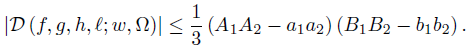
Proof. We use the following Ozeki’s type inequality obtained in [6]:

provided 0 < a1 ≤ f ≤ A1 < ∞, 0 < a2 ≤ g ≤ A2 < ∞ a.e. on Ω.
Since

when 0 < b1 ≤ h ≤ B1 < ∞, 0 < b2 ≤ ℓ ≤ B2 < ∞ a.e. on Ω, then by (20) we get the desired result (29).
4. Results for univariate functions
Let Ω = [a, b] be an interval of real numbers, and assume that f, g, h, ℓ : [a, b] →  are measurable D−Synchronous (D−Aynchronous), w ≥ 0 a.e. on [a, b] with
  w (t) dt = 1 and fh, gℓ, gh, fℓ ∈ Lw ([a, b]) ; then,
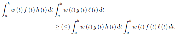 (30)
(30)
Now, assume that [a, b] ⊂ (0, ∞) and take f (t) = tp, g (t) = tq, h (t) = tr and ℓ (t) = ts with p, q, r, s ∈  . Then,
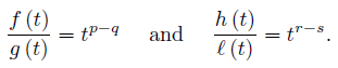
If (p − q) (r − s) > 0, then the functions  have the same monotonicity on [a, b] while if (p − q) (r − s) < 0 then
  have opposite monotonicity on [a, b] . Therefore, by (30) we have for any nonnegative integrable function w with
  w (t) dt = 1 that
 (31)
(31)
provided (p − q) (r − s) > (<) 0.
Assume that [a, b] ⊂ (0, ∞) and take f (t) = exp (αt), g (t) = exp (βt), h (t) = exp (γt) and ℓ (t) = exp (δt), with α, β, γ, δ ∈  . Then,
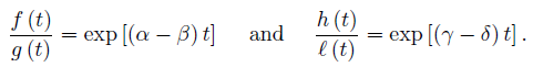
If (α − β) (γ − δ) > 0, then the functions  have the same monotonicity on [a, b] , while if (α − β) (γ − δ) < 0 then
  have opposite monotonicity on [a, b] . Therefore, by (30) we have for any nonnegative integrable function w with
  w (t) dt = 1 that
 (32)
(32)
provided (α − β) (γ − δ) > (<) 0.
Consider the functional
 (33)
(33)
for any nonnegative integrable function w with  w (t) dt = 1, and p, q, r, s ∈
  .
.
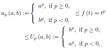
We observe that for t ∈ [a, b] ⊂ (0, ∞) we have
 (34)
(34)
and, similarly,

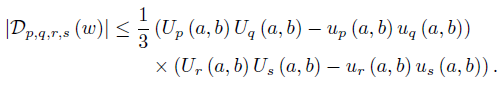
Using the inequality (22) we have
 (35)
(35)
while from (24) we have
 (36)
(36)
We also have for t ∈ [a, b] ⊂ (0, ∞) that
and the corresponding bounds for g (t) = tq, h (t) = tr and ℓ (t) = ts, with p, q, r, s ∈  . Making use of the inequality (29) we get
 (37)
(37)
Similar results may be stated for the functional
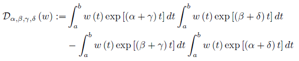
for any nonnegative integrable function w with  w (t) dt = 1, for α, β, γ, δ ∈
  and [a, b] ⊂ (0, ∞). Details are omitted.
We say that the function φ : [a, b] →  is Lipschitzian with the constant L > 0 if

for any t, s ∈ [a, b] .
Define the functional

In the next result we provided two upper bounds in terms of Lipschitzian constants:
Theorem 4.1. Let f, g, h, ℓ: [a, b] →  be measurable functions and w ≥ 0 a.e. on [a, b] with
 w (t) dt = 1.
(i) If g (t), ℓ (t)  0 for any t ∈ [a, b] , and
 is Lipschitzian with the constant L > 0, and is Lipschitzian with the constant K
 > 0, and gℓ, gℓe2 ∈ Lw ([a, b]) with e (t) = t, t ∈ [a, b], then
 (38)
(38)
(ii) If, in addition, we have wgℓ ∈ L∞ [a, b] and
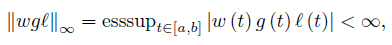
then
 (39)
(39)
Proof. We have

By taking modulus in this equality, we get
 (40)
(40)
Now, observe that
 (41)
(41)
On making use of (40) and (41) we get the desired result (38).
If wgℓ ∈ L∞ [a, b] , then
 (42)
(42)
Therefore, by inequalities (40) and (42) we obtain the desired result (39).
5. Discrete inequalities
Consider the n-tuples of real numbers x = (x1, ..., xn), y = (y1, ..., yn), z = (z1, ..., zn) and u = (u1, ..., un). We say that the quadruple (x, y, z, u) is D−Synchronous if
 (43)
(43)
for any i, j ∈ {1, ..., n} .
If p = (p1, ..., pn) is a probability distribution, namely, pi
≥ 0 for any i ∈ {1, ..., n} and  =1 pi = 1, and the quadruple (x, y, z, u) is D−Synchronous, then by (10) we have:
 (44)
(44)
For an n-tuples of real numbers x = (x1, ..., xn), we denote by |x| := (|x1| , ..., |xn|). On making use of the inequality (17), then for any D−Synchronous quadruple (x, y, z, u) and for any probability distribution p = (p1, ..., pn) we have
 (45)
(45)
Observe that if we consider
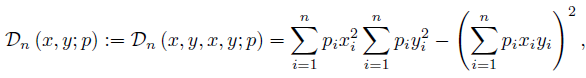
then by (20) we have
 (46)
(46)
for any quadruple (x, y, z, u) and any probability distribution p = (p1, ..., pn).
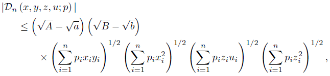
If a, A, b, B ∈  and (x, y, z, u) are such that A > a, B > b,
 (47)
(47)
for any i ∈ {1, ..., n} , then by (22) we have
 (48)
(48)
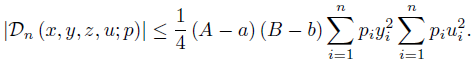
If a, A, b, B > 0 and condition (47) is valid, then by (24) we have
 (49)
(49)
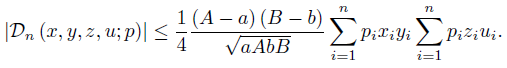
Now, if we use the Klamkin-McLenaghan’s inequality
that holds for x, y satisfying the condition (47) with A, a > 0, then by (46) we get
 (50)
(50)
provided (x, y, z, u) satisfy (47) with a, A, b, B > 0.
Now, assume that
 (51)
(51)
and
 (52)
(52)
for any i ∈ {1, ..., n} ; then by (29) we get
 (53)
(53)
for any probability distribution p = (p1, ..., pn ).

