


 English (pdf)
 Article in xml format
 Article references
 Send this article by e-mail
 Cited by SciELO
  Cited by Google
  Similars in
SciELO
Similars in
SciELO  Similars in Google
 Permalink
1. Introduction
Probably the simplest, most natural approach to constructing a homeomorphism is the following: Partition the spaces that are involved into finite sets, and then assign the sets in the first space to the sets in the second space in the manner desired. These partitions and set assignments give the first approximation to the homeomorphism. To obtain an improved approximation, partition the spaces again, obtaining refinements of the first partitions, and then assign sets to sets again, keeping these assignments consistent with those already made in the first step. Continue this process, getting at the n level partitions of the space that refine the partition chosen at the n − 1 level, and then assign sets to sets once more, being consistent with the choices already made. The homeomorphism approximation improves with each new level, and the end result (if all this is done with a fair amount of care) is a homeomorphism from the first space to the second which has the properties desired. This idea has been used by many topologists to construct homeomorphisms. See, for example, [4], [5], [15], [16], and [17].
This author has used this approach to construct self homeomorphisms that show that certain indecomposable continua can admit certain types of complicated dynamical behavior. (See [10], [11], [12], [13], and [14].) In this paper we would like to apply this idea in still another way. It can be used to give general topological proofs to some of the basic aspects of Carathéodory’s theory of prime ends. Since this theory has been used in a very powerful way by several dynamicists to obtain results about dynamics occurring in the plane ([3], [25], [2], and [20]), it is of interest now to topologists and dynamicists both, and it is perhaps worth noting that it can be justified using nothing more than some elementary facts from plane topology. Along the way we obtain a slight generalization to Carathéodory’s main theorem, and then obtain a Schoenflies theorem and a theorem of Rutt [24] as corollaries.
C. Carathéodory’s papers [6] and [7] on prime ends appeared in 1913 before there was a modern definition of a topological space. His theory concerns a certain compactification of open, connected sets on a surface. Suppose that E and E
◦
denote the closed and open unit disks in the plane, respectively. If D is an open, bounded, connected, simply connected subset of the plane, then there is a conformal mapping Φ of E
◦
onto D (Riemann mapping theorem). In his first paper on prime ends [6], Carathéodory obtained a conformal Schoenflies theorem: he proved that if the boundary of D in the plane is homeomorphic to a circle, then Φ extends to a homeomorphism of E onto
Other treatments of the theory of prime ends using conformal mapping machinery include those given by C. Pommerenke [23] and L. Ahlfors [1]. A treatment of the theory which relies on heavy analytic machinery is given in M. Ohtsuka’s book [22]. J. Mather [20] has given a very nice account of the theory which is largely topological, but his proofs make use of some not-stricly-topological structures (polyhedra and piecewise linear mappings, for example). M.H.A Newman [21] proved the Schoenflies theorem using topological methods, but his proofs do not use prime end theory. That is, of course, because he does not have to have it in the locally connected context. The basic construction involved in the treatment in this paper is a generalization of Newman’s.
Carathéodory’s theory has been used by many different kinds of mathematicians in many different ways. However, its applications in dynamics have brought it to the attention of this author. The power of the theory in this context comes about as follows: Suppose that D is an open, connected, bounded, simply connected plane region. Then D is homeomorphic to an open disk. Its boundary, though, need not be a simple closed curve, nor even anywhere close to being a simple closed curve. It is possible that it doesn’t even contain an arc. Then
Why then bother with yet another proof of the main results in the theory? In addition to the fact that a slight generalization of the theory is possible in this way, that one need only know general topology to understand it, and that a theorem of Rutt [24] is obtained as a corollary, it seems to this author to be worth noting exactly what assumptions, what structures are necessary to a given theory. Sometimes, for example, one of the things dynamicists wonder about is whether or not they can avoid some pathological behavior and pathological sets (pathological from their point of view, anyway) by making sufficient “nice” assumptions on the maps involved. Can they, for example, avoid indecomposable invariant continua by requiring C ∞ diffeomorphisms? Since they are concerned with the long term asymptotic behavior of the system, perhaps it is not terribly surprising that often the answer is “no” (see [9]). But what exactly is because of the topology and what is because of the other structures involved? In the case of the aspects of prime end theory that interest them, the answer is that it can all be put on an entirely topological basis. Another consideration is this: There have been some attempts to generalize prime end theory to higher dimensions, and thus far, it is the understanding of this author, they have not been very successful. Perhaps an approach that uses the least amount of structure possible has more of a chance at allowing generalization than do others.
The fundamental problem in showing that
However, even though the idea is quite simple, writing down the details in a sufficiently careful way to ensure that a proof really is there is quite tedious. Other authors have run into this problem, too. Mather [20] notes that, “It does not appear to be possible to give a brief account of Carathéodory’s theory which does not rely on some deep theory”. Although this account relies only on some basic facts from plane topology, and the ideas involved are not difficult, it cannot be called “brief” either.
2. Background, definitions, elementary facts.
We give here only the background needed for this exposition. The reader who is not already familiar with prime ends is referred to Mather’s very complete and very nice treatment [20] for more examples, more details, and a deeper understanding.
Suppose D is a connected, open set in the plane. (Actually, any open, connected subset of a surface will do. A surface is a Hausdorff topological space which has a countable basis and each point of which is contained in an open set homeomorphic to either the plane or the closed upper half plane.) A chain in D is a sequence
 of open connected subsets of D such that (i) V
1
⊇ V
2
⊇ . . .; (ii) ∂
D
V
n
≠ ∅ and connected for each n; and (iii)
of open connected subsets of D such that (i) V
1
⊇ V
2
⊇ . . .; (ii) ∂
D
V
n
≠ ∅ and connected for each n; and (iii)
 for n ≠ m. (Please note that a very important distinction is being made here. For B ⊆ A, ∂
A
B and Cl
A
B denote the boundary and closure of B in A, respectively. If X is the space containing A, then Cl
X
B = B and ∂
X
B = ∂B.) The chain
for n ≠ m. (Please note that a very important distinction is being made here. For B ⊆ A, ∂
A
B and Cl
A
B denote the boundary and closure of B in A, respectively. If X is the space containing A, then Cl
X
B = B and ∂
X
B = ∂B.) The chain
 is said to divide the chain
 provided that for each n, there is m such that W
m
⊆ V
n
. Two chains are equivalent if each divides the other. A chain is prime if every chain which divides it is equivalent to it.
provided that for each n, there is m such that W
m
⊆ V
n
. Two chains are equivalent if each divides the other. A chain is prime if every chain which divides it is equivalent to it.
A prime point of D is an equivalence class of prime chains of D. A prime end of D is a prime point of D with a representative prime chain
 such that ∂V
n
∩ ∂D # ∅ for all n. Let “D denote the collection of all prime points of D.
such that ∂V
n
∩ ∂D # ∅ for all n. Let “D denote the collection of all prime points of D.
Given an open set W in D and an element P of  of P has the property that V
n
⊆ W for some n. Let
of P has the property that V
n
⊆ W for some n. Let
(1) The collection W = {
(2) Convergence in this topology works as follows: lim n→∞ P n = P iff given a representative chain {V n } ∞ n=1 of P , for each m there exists N such that P n divides V m for all n ≥ N.
If P is a prime end of D with representative chain {V n } ∞ n=1 , the impression of P is I(P ) = ∩ ∞ n=1 V n . (Since I(P ) is the nested intersection of a collection of continua, I(P ) is a continuum. Further, since {V n } ∞ n=1 is prime, I(P ) ⊆ ∂D.)
If A is a subset of a topological space X, and p is a point of X, then p is accessible from the set A if there exists an arc P in X such that P ⊆ A ∪ {p} and p is an endpoint of P .
Suppose now that D is a bounded, simply connected, connected, open plane set. Let us list the elementary facts from plane topology that we will be using:
(1) An open arc is a set homeomorphic to (0,1). An open arc C in D is a cross-cut if ∂C consists of two distinct points in ∂D. Each cross-cut divides D into exactly two open sets, each of which is homeomorphic to an open disk. (In other words, each of these sets is itself a bounded, simply connected, connected, open plane set.)
(2) The set of points of ∂D that are accessible from D are dense in ∂D. (Although not crucial to our arguments, it is worth noting that ∂D (a) can be an indecomposable continuum, and (b) may not contain an arc, even though it does have to be connected. For example, it could be a pseudocircle. Then a theorem of S. Mazurkiewicz tells us that the set of points of an indecomposable continuum in the plane that are accessible from the plane minus the continuum is a first category subset of the indecomposable continuum. Thus, the accessible points of ∂D may well be a rather small subset of the continuum, although a dense subset.)
(3) If A is an arc in D, then every point of A is accessible from D \ A.
(4) If D is an arcwise connected subset of the plane, then D is simply connected provided that if S is a simple closed curve contained in D, then the bounded component of the complement of S in the plane is contained in D. This is equivalent to saying that if S is a continuous image of a simple closed curve contained in D, then each bounded component of the complement of S in the plane is contained in D.
Note that if {V n } ∞ n=1 is a prime chain in D representing a prime end P , there is a sequence of cross-cuts {C n } ∞ n=1 such that
(a) C n ⊆ V n ;
(b) C n separates D into two connected, open sets, one of which -call it U n - is contained in V n ; and
(c) {U n } ∞ n=1 is a prime chain equivalent to {V n } ∞ n=1 .
We will say that {C n } ∞ n=1 is a representative sequence of cross-cuts for the prime end P .
We will need the following facts, the first one is a simple result of general topology and we leave the proof to the reader, the other two are proved in Mather’s paper.
Lemma 2.1. Suppose X is a connected topological space, and A and B are nonempty, connected, open subsets of X whose boundaries are nonempty, connected, and disjoint. Then one of the following is true: X = A ∪ B, A ⊆ B, B ⊆ A, or A ∩ B = ∅.
Theorem 2.2 ([19], Lemma 3.2). Suppose σ = {V 1 , V 2 , . . .} and τ = {W 1 , W 2 , . . .} are two chains of the surface S. Further, suppose that for each open set O that contains the point x of S, there exists n 0 such that ∂ D V n ⊆ O for n ≥ n 0 , and that V i ∩ W j # ∅ for all i, j. Then σ divides τ.
Corollary 2.3 ([19], Corollary 3.3). If σ = {V 1 , V 2 , . . .} is a chain such that {∂ D V n } ∞ n=1 converges to a point in the surface S, then σ is prime.
If x ∈
Let us caution the reader about one thing: in general, there are no simple relationships between the impressions of prime ends, the principal sets of prime ends, and the prime ends themselves. The impressions do not generally give a collection of mutually disjoint continua in the boundary, for example. For a given prime end P, the impression and principal set are always nonempty, but beyond noting that the impression always contains the principal set, not much can be said. It is possible that one continuum is the impression for two different prime ends, too. For more explanation of these matters, see [20].
If X is a compact metric space and C = {c(0), c(1), . . . , c(m)} is a finite cover of X which consists of closed, regular neighborhoods, then C is a tiling iff c(i) ∩ c(j) = ∂c(i) ∩ ∂c(j) for each i # j in {0, 1, . . . , m}. (A closed neighborhood B is regular if (
Theorem 2.4. Suppose that X and Y are compact metric spaces and G 1 , G 2 , . . . and H 1 , H 2 , . . . are sequences of tilings of X and Y , respectively, such that
(1) for each i, G i = {g(i, 0), g(i, 1), . . . , g(i, a(i)))} and H i = {h(i, 0), h(i, 1), . . . , h(i, a(i)))};
(2) if A ⊆ {0, 1, . . . , a(i)}, then ∩ j∈A g(i, j) ≠ ∅ iff ∩ j∈A h(i, j) ≠ ∅;
(3) lim i mesh G i = lim i mesh H i = 0; and
(4) for each i, G i+1 follows the pattern η i in G i and H i+1 follows η i in H i .
Then for x ∈ X, there is an infinite sequence j(x, 1), j(x, 2), . . . of integers such that
(1) x ∈ g(i, j(x, i)), and
(2) η i (j(x, i + 1)) = j(x, i).
Further, if we define
 , then T: X → Y is a homeomorphism.
Proof. We will not give his proof here. We leave it as an exercise for the reader, or refer him/her to [10, Theorem 1].
A continuous function f: X → Y is confluent if the preimage of each continuum K in Y is a collection of continua in X each of which maps onto K. The continuous function f is monotone if the preimage of each continuum K in Y is a continuum in X. Clearly,
(1) monotone maps are confluent;
(2) there are many monotone self maps on connected open plane sets that are not homeomorphisms;
(3) there are many confluent self maps on connected open plane sets that are not monotone.
3. Statements and proofs of the theorems.
Theorem 3.1.
Suppose D is an open, bounded, connected subset of the plane whose boundary is connected. Then
(1) a homeomorphism β:
(2) an extension
(3) a surjection G: E → E such that β
Proof. Note that the collection of accessible points on ∂D is not only dense, but it is also the case that if O is an open set in the plane that intersects the boundary of D, then each component of D ∩ O contains a point accessible from D. Further, given two different accessible points of ∂D, there are two different prime ends associated with those two points. Choose a countable dense subset P of ∂D as follows: For each n ∈ ℕ, there is a finite cover of ∂D by connected, open sets of diameter less than 1/n. If O denotes one member of this collection, then O ∩ D has at most a countable number of components. For each of these components choose a point in ∂D accesible from the component. Let Pn denote the resulting collection of accessible points. Note that Pn S
∞
is countable. Let
 , so that P is a countable dense subset of ∂D with the desired property.
Next choose a countable dense subset Q of ∂E. List both P and Q as follows: P = {p 0 , p 1 , . . .} and Q = {q 0 , q 1 , . . .}. Then choose a point p in D ◦ and let q = (0, 0) in E ◦ . Next choose an arc A 0 from p to p 0, and an arc A 1 from p to p 1 such that A 0 ∩ ∂D = {p 0 }, A 1 ∩ ∂D = {p 1 }, and A 0 ∩ A 1 = {p}. In E, let B 0 and B 1 denote the intersection of the rays from q through q 0 and q 1, respectively, with E.
Now choose a closed disk D 1/2 in D so that
(1) p ∈ D 1/2 ◦ ; and
(2) ∂ D D 1/2 ∩ A 0 and ∂ D D 1/2 ∩ A 1 consist of exactly one point.
Let E 1/2 = {x ∈ E | ∥x∥ ≤ 1/2}.
What do we now have? Each of D ∪ P and E ∪ Q has been divided by A 0 , A 1, and D 1/2 ; and B 0,
(3) Each region is connected and closed (in D ∪ P or E ◦ ∪ Q).
(4) The interior of each region is an open disk, topologically.
(5) The regions in D ∪ P are listed as G 1 = {g(1, 0), g(1, 1), g(1, 2), g(1, 3)}.
(6) The regions in E ◦ ∪ Q are listed as H 1 = {h(1, 0), h(1, 1), h(1, 2), h(1, 3)}.
(7) There is a “natural” correspondence between the four regions, and this is reflected in the listings. (By this we mean the following: g(1, i) ≅ h(1, i)) and if A ⊆ {0, 1, 2, 3}, then ∩ n∈ Ag(1, i) # ∅ iff ∩ n∈ Ah(1, i) # ∅.)
Let C(1) = {p 0 , p 1 } and C ′ (1) = {q 0 , q 1 }. Next choose finite subsets C(2) and C ′ (2) of P and Q as follows:
(8) |C(2)| = |C ′ (2)| with C(2) ⊆ P \ C(1) and C ′ (2) ⊆ Q \ C ′ (1);
(9) p 2 ∈ C(2) and q 2 ∈ C ′ (2);
(10) C(2) = {p 2,0 , p 2,1 , . . . , p 2,m(2) } and C ′ (2) = {q 2,0 , q 2,1 , . . . , q 2,m(2) };
(11) for i ∈ {0, 1, 2, . . . , m(2)} there is an arc A 2,i from p to p 2,i in D such that A 2,i ∩ ∂D = {p 2,i }, A 2,i ∩ ∂D 1/2 consists of exactly one point, and A 2,i ∩ A 0 = {p} = A 2,i ∩ A 1;
(12) for i ∈ {0, 1, 2, . . . , m(2)} there is a ray B 2,i from q to q 2,i in E ◦ such that B 2,i ∩ ∂E = {q 2,i }, B 2,i ∩ E 1/2 consist of exactly one point, and B 2,1 ∩ B 0 = {q} = B 2,i ∩ B 1; and
(13) for i, j ∈ {0, 1, 2, . . . , m(2)}, A 2,i ∩ A 2,j = {p}.
Note that a natural, circular ordering of the points of not only Q, but also of P , is being set up, and the listing and choice of points in C(2) and C ′ (2) reflects this: Let A 1,0 = A 0 and A 1,1 = A 1. Each arc A 2,j chosen splits one of the open disks in the collection of open disks that make up D\ ∪{A 1,0 , A 1,1 , A 2,1 , . . . , A 2,j−1 } into exactly two open disk. If A k,1 and A k ′ ,1 ′ denote the arcs bounding the split disk, we may, without ambiguity, consider p 2,j to be between p k,1 and p k ′ ,1 ′ . Likewise (and in a simpler manner) q 2,j will be chosen so that q 2,j is between q k,1 and q k ′ ,1 ′ . Thus,
(14) |C(2) ∩ g(1, i)| = |C ′ (2) ∩ h(1, i)| for i ∈ {0, 1, 2, 3}. D 1/4 and D 3/4 in D such that p ∈ D 1/4 ◦ ⊆ D 1/4 ⊆ D 1/2 each point of D 3/4 is within a distance of 1/4 from ∂D. Having done this, choose closed disks ⊆ D 1/2 ⊆ D 3/4 ◦ ⊆ D 3/4 ⊆ D, and Let E 1/4 = {x ∈ E | ∥x∥ ≤ 1/4},
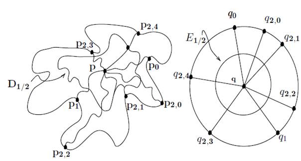
E 3/4 = {x ∈ E | ∥x ∥ ≤ 3/4}. Further, choose the disks D 1/4 and D 3/4 so that the boundary of each intersects each of the arcs A i,j exactly in one point. Note that the collection of all arcs A i,j and disks D r thus chosen partitions D ∪ P into a finite collection of relatively closed, connected, simply connected sets that intersect only at their boundaries in D ∪ P , and that the collection of all rays B i,j and disks E r thus chosen partitions E ◦ ∪ Q into a finite collection of relatively closed, connected, simply connected sets that intersect only at their boundaries in E ◦ ∪ Q. See Figure 1. Further, there is a natural correspondence between these collections of sets, which we will name G 2 = {g(2, 0), g(2, 1), . . . , g(2, n(2))} and H 2 = {h(2, 0), h(2, 1), . . . , h(2, n(2))} for D ∪P and E ◦ ∪ Q, respectively, such that
(15) if γ ⊆ {0, 1, . . . , n(2)}, then ∩ i∈γ g(2, i) #∅ iff ∩ i∈γ h(2, i) ≠ ∅ and
(16) each g(2, i) ≅ h(2, i).
Also, G 2 refines G 1 and, therefore, follows some pattern η 1 in G 1. The collection H 2 follows the same pattern η 1 in H 1
Continue the process that has been started, choosing two sequences G 1 , G 2 , . . . and H 1 , H 2 , . . . of collections of covers of D ∪ P and E ◦ ∪ Q, respectively; two sequences C(1), C(2), . . . and C ′ (1), C ′ (2), . . . of subsets of P and Q, respectively; two sequences A(1) = {A 1,0 , A 1,1 }, A2 = {A 2,0 , . . . , A 2,m(2) }, . . . and B(1) = {B 1,0 , B 1,1 }, B (2) = {B 2,0 , B 2,1 , . . . , B 2,m(2) }, . . . of arcs in D∪P and rays in E ◦ ∪ Q, respectively; ⅅ = {D r | r is a dyadic rational in (0, 1)}, a collection of closed disks in D; and E = {E r | r is a dyadic rational in (0, 1)}, where E r = {x ∈ E | ∥x∥ ≤ r}, so that
(17) G i+1 follows the pattern η i in G i , and H i+1 follows the pattern η i in H i ;
(18) we list G i = {g(i, 0), g(i, 1), . . . , g(i, n(i))} and H i = {h(i, 0), h(i, 1), . . . , h(i, n(i))};
(19) each member of P is in some C(i) and each member of Q is in some C ′ (i);
(20) each C(i) is finite and |C(i)| = |C ′ (i)|;
(21) each arc A i,j intersects ∂D in exactly the point p i,j in C(i) = {p i,1 , . . . , p i,m(i) }, intersects the boundary of the disk D r in exactly one point, and intersects any other arc A k,1 in exactly the point p;
(22) ∪D r = D with each point of the boundary of D (2 n −1)/2 n within a distance of 1/2 n from ∂D;
(23) each ray B i,j intersects ∂E in exactly the point q i,j ; and
(24) if r and r ′ are dyadic rationals in (0,1) and r < r ′ , then D r ⊆ D r ′ ◦ .
We may also, without loss of generality, require that the following properties hold:
(25) lim i→∞ mesh {g(i, j) ∈ G i | g(i, j) ⊆ D r } = 0, for r a fixed dyadic rational in (0,1).
(26) lim i→∞ mesh {g(i, j) ∩ A k,i | g(i, j) ∈ G i } = 0 (for fixed A k,1 ).
Finally then, we may define a map β: P ∪ D → Q ∪ E ◦ as follows: If x ∈ D ∪ P , then there is an infinite sequence j(x, 1), j(x, 2), . . . of integers such that for each i
(27) x ∈ g(i, j(x, i)), and
(28) η i (j(x, i + 1)) = j(x, i). Define β(x) = ∩ i∈N h(i, j(x, i)). It is not difficult to check that β is well-defined, one-to-one, and onto. Further, because of the fact that if X = D r for some allowable r, or X = A k,l for some allowable k and l, then G i (X) = {g(i, j) ∩ X | j ∈ {0, . . . , n(i)}} and g(i, j) ∩ X # ∅} is a tiling on X, and H i (X) = {h(i, j) ∩ β(X) | (g(i, j) ∩ X) ∈ G i (X)} is a tiling on β(X), and the fact that the tilings involved satisfy the requirements of the background theorem given, it follows that β| X : X → β(X) is a homeomorphism. Also, β(g(i, j)) = h(i, j), β(A k,l ) = B k,l , β(D r ) = E r , and β(p k,1 ) = q k,l (for appropriate i, j, k, l, and r). Then β| D : D → E ◦ is a homeomorphism.
β is also continuous: Suppose q m,1 ∈ Q and O is an open set in E that contains q m,1 . Then there is some h(i, j) in some H i such that q m,l ∈ h(i, j) ◦ and h(i, j) ⊆ O. Since p m,l ∈ g(i, j) ◦ and if x ∈ g(i, j), then β(x) ∈ h(i, j), it follows that β is continuous on D ∪ P .
We have now a map from D to E
◦
that is “sufficiently nice”. That is, if P is a prime end in  is an arc whose endpoints are two points in P , that intersects ∂D only in those two points, and such that
 is a homeomorphism.
By construction, {β(Vn)}
∞
n=1
is a prime chain in
 . If we define,
 , the prime end represented by
 is well-defined, and it is a simple matter to check that it is in fact a homeomorphism.
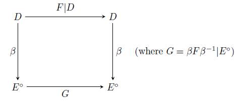
Let us turn our attention then to F . Note that the diagram below commutes:
Suppose {V
n
}
∞
n=1
is a prime chain in D chosen so that lim
n
diam(∂
D
V
n
) = 0, and lim
n
∂
D
V
n
= {x}. Then {F (V
n
)}
∞
n=1
is a nested collection of connected sets in D, as is
 . For each x in D. let ϵ
x
= min{∥x − y∥ | y ∈ ∂D}/2, and let B
ϵ
(z) denote the ϵ-ball about the point z in the plane. For each positive integer n, let W
n
= ∪{B
ϵx/2n
(x) | x ∈ D ∩ F (V
n
)}. Hence, W
n
is connected and open in D, and {W
n
}
∞
n=1
is a chain, but is it a prime chain?
. For each x in D. let ϵ
x
= min{∥x − y∥ | y ∈ ∂D}/2, and let B
ϵ
(z) denote the ϵ-ball about the point z in the plane. For each positive integer n, let W
n
= ∪{B
ϵx/2n
(x) | x ∈ D ∩ F (V
n
)}. Hence, W
n
is connected and open in D, and {W
n
}
∞
n=1
is a chain, but is it a prime chain?
Note that if W is a connected, open set of  . Suppose that the chain {W
n
′
}
∞
n=1
divides {W
n
}
∞
n=1
. Without loss of generality, we may assume that Cl
D
W
n
′
⊆ W
n
and that F (V
n
) ∩ W
n
′
≠ ∅. Let K
n
′
denote that component of F
−1
(W
n
′
) that intersects V
n
. Now {K
n
′
}
∞
n=1
is a chain in
. Suppose that the chain {W
n
′
}
∞
n=1
divides {W
n
}
∞
n=1
. Without loss of generality, we may assume that Cl
D
W
n
′
⊆ W
n
and that F (V
n
) ∩ W
n
′
≠ ∅. Let K
n
′
denote that component of F
−1
(W
n
′
) that intersects V
n
. Now {K
n
′
}
∞
n=1
is a chain in  , we are done.
Theorem 3.2.
(Schoenflies) Suppose that D is a bounded, connected, regular, open subset of the plane, that ∂D is locally connected, and that
Proof. Please recall the proof and construction given for Carathéodory’s Theorem, as we refer to it here and give the notation used the same meaning.
First, in the countable dense subset P of ∂D that was chosen, a circular ordering was set up on the members of P . In particular, note that whenever p
m,1
= a and p
m
′
,1
′ = a
′
are members of P , suppose T denotes an arc in ∂D with endpoints a and a
′
. Since A
m,1
∪ T ∪ A
m
′
,1
′ = T
′
is a simple closed curve in D, the bounded component C of the complement of T
′
is contained in D. Let U
1 and U
2 denote the components of D \ (A
m,1
∪ A
m
′
,1
′ ). Either C ⊆ U
1 or C ⊆ U
2, say C ⊆ U
1. Then ∂
D
C = ∂
D
U
1. Each radial arc A
r,s
, besides A
m,1
and A
m
′
,1
′ , intersects either U
1 or U
2. Since ∂
D
C = ∂
D
U
1, any radial arc that intersects U
1 also intersects C. Then it is contained, except for its endpoints, in C. It follows that C = U
1 (because C is dense in U
1 and U
1 is regular), and T
′
=
Further, since ∂D is locally connected, and therefore points close together in P may be connected with arcs of small diameter, we may choose a finite subset {a(0), a(1), . . . , a(n)} of P , with a(0) = p 0 < a(1) < · · · < a(n), such that each pair a(i), a(i + 1) is connected by an arc T (i) in ∂D whose endpoints are a(i) and a(i + 1), and such that each T (i) contains each point in P “between” a(i) and a(i + 1). Further, we may choose this set so that an arc T (n) in ∂D whose endpoints are a(n) and a(0) contains every point “between” a(0) and a(n) in P . Then ∪T (i) = ∂D. Let C(i) denote the bounded component of the complement of the simple closed curve formed by T (i) and its associated radial arcs. Suppose T (i) ∩ T (j) # ∅. Without loss of generality, we may assume that j = i + 1. (If not, we can combine any intervening arcs, and lose nothing.) Now T (i) ∩T (i + 1) does at least contain the common endpoint a(i + 1), but suppose there is another point in the intersection.
Suppose the point t ≠ a(i + 1) is in the intersection, and that n > 1. There are points p m,1 , p m ′ ,1 ′ , and p k,r in P such that the ends of T (i) are p m,1 and p m ′ ,1 ′ , and the ends of T (i + 1) are p m ′ ,1 ′ and p k,r . Now p m,1 < p m ′ ,1 ′ < p k,r . Let [p m,1 , t] and [t, p m ′ ,1 ′ ] denote the subarcs of T (i) determined by t, and let [p m ′ ,1 ′ , t] and [t, p k,r ] denote the subarcs of T (i + 1) determined by t. (It is possible that one of these “arcs” is degenerate.) Now we may assume that S(1) = A m,1 ∪ [p m,1 , t] ∪ [t, p k,r ] ∪ A k,r is a simple closed curve. However, [t, p m ′ ,1 ′ ] ∪ [p m ′ ,1 ′ , t] = S(2) is the continuous image of a simple closed curve which is nondegenerate and intersects S(1) in exactly the point t. But this is impossible : The bounded component of the complement of S(1) contains C(i) ∪ C(i + 1), and so p m ′ ,1 ′ ∈ S(1) ∩ S(2). However, p m ′ ,1 ′ ∈/ S(1).
By construction, for the case where ∂D is locally connected, β
−1
: E
◦
∪ Q → D ∪ P is a home-omorphism, for in this situation, lim
i
mesh G
i
= 0. In fact, we may go even further: Let
 . Then each
  , and that ∂g(i, j) ∩ ∂g(i
′
, j
′
) ∩ ∂D = ∅ or consists of one point of P .)
, and that ∂g(i, j) ∩ ∂g(i
′
, j
′
) ∩ ∂D = ∅ or consists of one point of P .)
Theorem 3.3.
(Rutt [24], Theorem 4) If ∂D is and indecomposable continuum, then there is a prime end P in
Proof. Again, this proof refers to the construction and notation of the Carathéodory Theorem. For each i, there is some g(i, j) ∈ G i such that ∂g(i, j) ∩ ∂D is an indecomposable continuum. (Otherwise ∂D is the union of a finite number of nowhere dense subcontinua.) Then we can find an infinite nested sequence g(1, i 1) ⊇ g(2, i 2) ⊇ . . . so that each g(k, i k ) contains ∂D in its boundary in the plane. This sequence {g(k, i k )} ∞ k=1 may not be a chain, however, for it is possible that the boundaries of two different members of the sequence intersect in D. We can correct this by considering r(i) = {g(i, j) ∪ g(i, k) | g(i, j) and g(i, k) are adjacent members of G i with points of ∂D in their closure}. Then we may obtain an infinite sequence {r(i)} ∞ i=1 such that for each i and j ∈ ℕ:
(1) ∂D ∩ ∂r(i) is an indecomposable continuum;
(2) Cl D r(i + 1) ⊆ r(i); and
(3)

By construction, it also follows that {r(i)}
T
∞
i=1
is a prime chain. (Remember the map β and the associated chain
 Thus,
Thus,
 , where P is the prime end represented by {r(i)}
∞
i=1
.
, where P is the prime end represented by {r(i)}
∞
i=1
.


