


 English (pdf)
 Article in xml format
 Article references
 Send this article by e-mail
 Cited by SciELO
  Cited by Google
  Similars in
SciELO
Similars in
SciELO  Similars in Google
 Permalink
1. Introduction
The Optimality Criteria (OC) methods trace their origin to intuitive traditional approaches to the problem of strength design, more directly to the Fully Stress Design (FSD) criteria, with its associated stress ratio resizing algorithm. The FSD criterion states that a structure is of minimum weight if every member is at its maximum allowable stresses, or at its minimum size at least under one of the loading conditions. This criterion is based on the intuitive, yet incomplete assumption that if a structure is sized so as not to fail either locally or globally under its critical loads, then that structure must be optimum [1]. Later on, the procedures characterized as mathematics programming formulations appeared on the scene. To define them in a succinct way, they look for the minimum or maximum, depending on the objective function, of a multi-variable function subject to limitations (restrictions) expressed by equalities or inequalities. The representation of inequality constraints is important as it allows for identifying the design as that in which not all the elements are subject to limited conditions under a load system. This avoids a limitation that is inherent in some of the above methods. The idea of characterizing an optimum structure through conditions that are believed to exist at an optimum and then applying a resizing procedure that directly satisfies those conditions is the fundamental approach normally used by those designers which became formalized as the Optimality Criterion methods, which are classified as parametric structural optimization. Such Optimality criterion consists of discretizing a pre-established structure to find the optimal dimensions of the structure. The design variables that can be modified are the cross-sectional area of each element, lengths, thicknesses and notch radii, unlike topological optimization where holes or cavities are introduced in the structure that were not present at the beginning.
In [2] and [3] it is used an optimality criteria method that proposed a uniform distribution of strain energy in optimal trusses. In [4] it is derived an optimality criterion based on the Kuhn-Tucker conditions for problems with a single restriction, yet unfortunately, it was inapplicable to problems with multiple restrictions. In the 1970-1980 decades, several authors propose various algorithms to identify active restrictions based on the estimation of Lagrange multipliers of the Kuhn-Tucker conditions in problems with multiple restrictions. A unifying vision of all of them is offered in [5,6] and [7]. However, the problems inherent in the active restrictions identifying methods were not solved rigorously until the development of the dual formulation, in which the identification of active constraints was substantial and intimately linked to the algorithm of mathematical programming used to solve the problem of minimization. From this moment on, the dual formulation was the unifying link between the Optimality Criterion and the mathematical programming techniques. It should be noted that so far, algorithms based on dual formulation, such as the OC does, have only been able to test its effectiveness in structural optimization problems where the optimum is conditioned by a relatively low number of restrictions [6].
There are several works related to optimality criteria in structural design; for example, the work by [8] where the optimality criterion is applied to the design of lattice structures, the work by [9] using a different resizing rule on the design of laminated composites. In the present work, the optimality criterion is used in the design of truss structures implementing the linear resizing rules with n g = 1 and n g = 2 constraints. They can be implemented with more constraints, taking into account the loss of effectiveness of the method in the face of a high number of restrictions. The constraints formulation is obtained from the statics of the structure, in this case, an indeterminate structure, in which Equations of static equilibrium are not sufficient to determine all the forces and reactions. The resizing rules presented in this work are based on the assumption that the load distribution in the structure is independent of the member sizes and that the loads carried by the members remain constant. So, the linear resizing rule is used to determine the optimal design variables in such a way that minimize the objective function satisfying the restrictions.
2. Description of the mechanical model
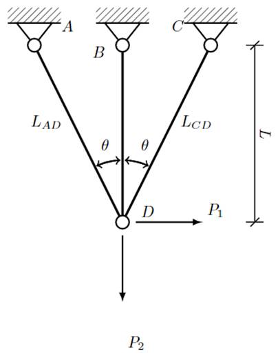
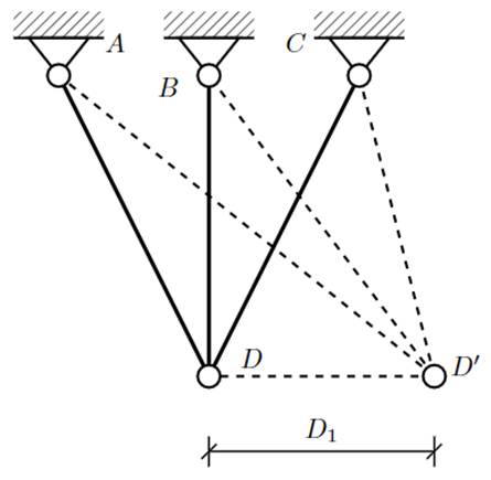
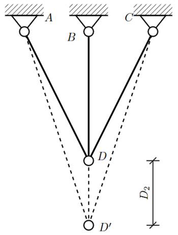
Figure 1 shows the mechanical system analyzed herein. The sectional areas and normal stresses in the lateral bars between nodes A-D, B-D and C-D are A AD , A BD , A CD and σ AD , σ BD , σ CD , respectively. The A-D and C-D lateral bars show rotations θ 1 and θ 2 with respect to the vertical B-D. The B-D bar features length L, and the lateral bars feature lengths LAD = L/ cos (θ 1), L CD = L/ cos (θ 2). All the bars are built from the same linearly elastic material featuring modulus of elasticity E. It is clear that the truss has only two degrees of freedom for joint translation, namely the D 1 and D 2 horizontal and vertical translations at joint D, as shown in Figures 2 and 3.
By applying Castigliano’s first theorem to the strain energies of the displacements D1 and D2 [10], we obtain the following Equations (1) and (2) for the joint displacements:

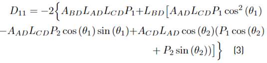
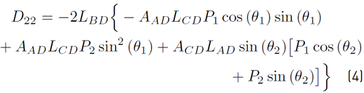
where D 11, D 22 and D∗ are presented in equations (3), (4) and (5)

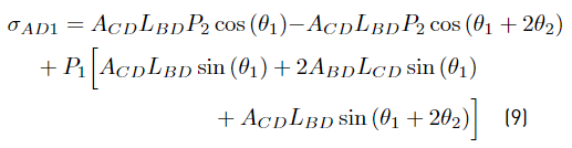
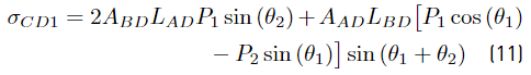
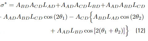
and the stresses in the bars in Equations (6), (7) and (8)
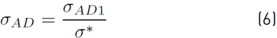
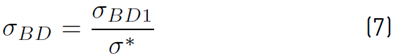
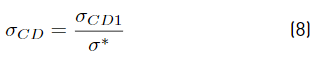
where σ AD1 , σ BD1 , σ CD1 and σ∗ are shown in Equations (9), (10), (11) and (12).

2.1 Definition of the optimization model
The combination of the P 1 and P 2 forces can represent the components of any force acting on node D; however, only positive forces are considered here according to the directions described in Figure 1. The presence of the positive P 1 and P 2 forces implies that the normal stressin the A-D bar is always Positive, but the stress in the C-D bar can be positive or negative. For the sake of model reduction, some symmetries are introduced: the sectional areas and rotation angles of the lateral bars of the A-Dand C-D nodes are equal; they are A AD = A CD and θ AD = θ CD respectively. The new design variables are x 1 = A AD 0.002E, x 2 = ABD0.002E, θ = θ AD = θ CD . The optimization problem consists of finding a minimum-mass design for the truss, given by (13)

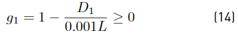
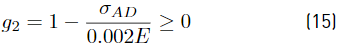
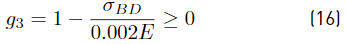
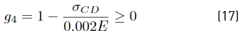
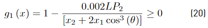
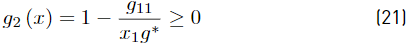
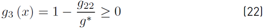
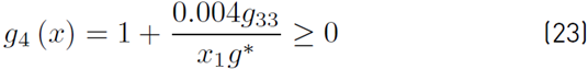
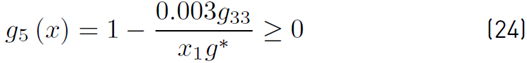
where ρ is the mass density. The truss is designed in subjection to 5 constraints shown in Equations (14) to (18); g 1 corresponds to the vertical displacement at node D and can not exceed a value of D 2max = 0.001L. The g 2 to g 4 constraints are related to limits on the traction stresses σ t max = 0.002E and finally g 5 is related to compression stress limit in the bar C-D σ c max = 0.0015E

Considering the previous reductions, the design problem may be rewritten as Equations (19) - (24)

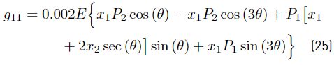
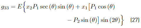
where g11, g22, g33 and g∗ are presented in Equations (25)-(28)


3. Optimization algorithm
The optimization problem can be represented by (29)

In this work the objective function is linear. For these problems the Kuhn-Tucker condition is (30)

In terms of the original design variables, Equation (30) becomes (31)
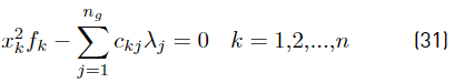
where fk and ckj are presented in (32)

3.1 Resizing approximation rules
Another possibility for rewriting eq 31 is the exponential rule (33)
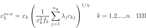
where the old value for x k is used to produce a new estimate. A linearized form of eq (33) obtained by binomial expansion is presented in (34)

where Δxk and λj are described in (35) and (36)
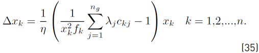

the term η is a step size parameter. This linearized form is known as the linear resizing rule.
3.2 Upper and lower limits on design variables
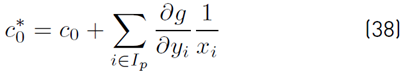
In many cases, it is necessary to have lower and upper limits on design variables besides the displacement constraints. The set of design variables that are at their lower or upper limits during iterations is called the passive set, I p , while the set including the rest of the variables is called the active set, I a . Such design variables call for some modifications on the resizing algorithm. Thus, the Lagrange multiplier λ is shown in Equation (37)
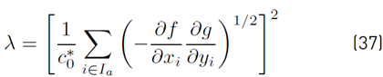
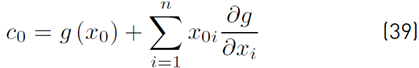
where c∗ 0 and c 0 are presented in (38) and (39)
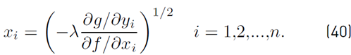
and the resizing Equation (40) is obtained from Equation (31)
4. Results
This section shows the results obtained by the linear resizing rule with and without limits on the design variables. Two different cases are considered depending on the θ angle, the P 1, P 2 loads and the objective function in order to adapt the models to those presented in [6] and [7]. The first example, from [6], shows the results of a three-bar truss with the objective function (41)
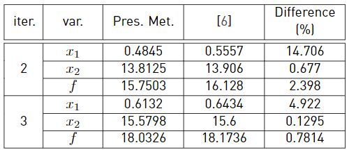
and two restrictions: the vertical displacement and the stress in the A-D bar; these are Equations (19) and (21). This example also considers P 2 = 8P 1, θ = π/3 and x 0 = (1, 10) T as a starting point. The reference shows the results only for the first three iterations. They are shown in Table 1 below, where the maximal difference between [6] and the results obtained here is 14.7% at the first iteration when estimating x 1. Figures 4 and 5 show the plotted values for the first 10 iterations. It widely shows the fast convergence to the limit values of x 1 = 0.6598, x 2 = 15.835 and a cost function f = 18.474358.

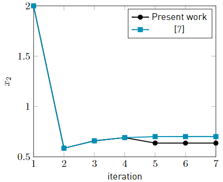
The second three-bar truss optimization structure is presented by [7]. This optimization problem considers a D 2max = 0.001 inch displacement restriction on the vertical direction, with equal forces P 1 = P 2 = 300/ √2 lb in the vertical and horizontal directions, θ = π/4 angle of rotation of the lateral bars, ρ = 0.283 lb/in3 density, E = 30 × 106 psi elsaticity modulus, L = 100√2 inch length and x 0 = (2, 2) T as starting point. So, the design variables are x 1 = A AD E/P1l = A CD E/P 1 l and x 2 = A BD E/P 1 l. Two lower limits in the design variables x 1 ≥ 0.1 and x 2 ≥ 0.1 are considered in [7]. The present work considers only the x 1 ≥ 0.1 limit as a passive restriction. The results for the first seven iterations are shown in Table 2. Figure 6 plots the first 7 x 2 iteration values presented by [6] with a blue squared line, and the values here obtained with a black dotted line.

5. Conclusions
The results of the first example shown in Figures 4 and 5 were computed in 0.125364 seconds. The Matlab Optimization Toolbox was used to solve this example as well, and, after 34 iterations in 9.2498 seconds, the results were x 1 = 0.6598288, x 2 = 15.852457 and f = 18.491773. The analytical solution of this example can be found by equalling both constraints to zero and solving the system for the variables; when doing so, these results are x 1 = 0.659726, x 2 = 15.8525 and f = 18.4914. This example displayed a fast convergence of the reciprocal exponential resizing rule, as expected, because there are only two restrictions, and both of them are of the passive type.
Regarding the second example, Figure 6 shows a separation between the plot lines from the 5th iteration; such difference is around 0.101%. The difference in the values of the cost function is remarkable. The results for the 7th iteration by [7] are f = 27.847560; for the values here presented, they are f = 26.014459, the difference being 6.58%.
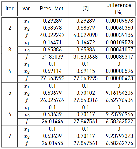
Therefore, it can be said that this work proposes a better cost function with less computation effort. Because the results were known a priori, a conclusion was reached that the optimal solution has the tendency to take the lowest limit in x 1, but not in x 2, only the x 1 boundary was included in this work’s optimization model. The Matlab Optimization Toolbox was used to solve this example as well, and after 27 iterations in 9.4198 seconds, the results were f = 26.014458, x 1 = 0.1 and x 2 = 0.636396.

