


 English (pdf)
 Article in xml format
 Article references
 Send this article by e-mail
 Cited by SciELO
  Cited by Google
  Similars in
SciELO
Similars in
SciELO  Similars in Google
 Permalink
Introduction
Vision-based measurement (VBM) systems use cameras as an instrument 1. This emerging trend is becoming increasingly popular as an affordable and suitable alternative for many applications such as on-road vehicle detection, tracking, behavior understanding 2, robotics 3, physics 4, biology 5, and engineering 6.
This work introduces a method to calculate acceleration from a real uniformly accelerated motion-blurred image. It uses homomorphic mapping to extract the characteristic point spread function (PSF) of the degraded image, in order to train a machine learning regression model with 125 known instances and responses that finally predicts acceleration as a regression. This approach considers the motion angle to be equal to zero, even though constant acceleration is obtained from an inclined slider. The ground-truth acceleration of each blurred image was measured independently since the sliding camera platform’s friction could slightly change the acceleration from measurement to measurement.
Homomorphic filtering is widely used in several applications, as shown in7) (8, and 9. Although image restoration based on homomorphic filtering is a usual task in image processing, this approach has not been proposed in the literature for acceleration estimation. Homomorphic filtering objectively enhances the image but does not calculate acceleration in the filtering process.
There are two classes of acceleration measurement techniques. The first one involves direct measurements carried out by accelerometers without the need for individual calculations. These accelerometers can be classified based on their operation principle: the piezoelectric effect, the capacitive effect, microelectromechanical systems (MEMS), and the electromechanical servo principle. Some drawbacks of this class are that they are range-fixed, more expensive, and invasive. Direct measurement accelerometers usually need wires that run from the moving target to the analysis system. In some cases, cables can negatively influence the action measured 4. The second class is indirect measurements, where acceleration is estimated from another kinematic variable, using circuits or a computational algorithm.
Kinematic quantities, such as acceleration, are related to the forces that engineering structures can support 10. For instance, some constructions such as floors, footbridges, buildings, and bridges must be continually monitored to evaluate their structural safety 11. Usually, motion sensors need to be connected to a monitoring system, which is often hard to place due to wiring and power issues. Some vision-based displacement measurement systems have been recently developed for structural monitoring because they overcome the already listed issues 16) (12.
Motion, velocity, and acceleration are related to kinematic quantities through time. This means that it is possible to obtain one from another via integration or differentiation. The differential of displacement is called velocity, and the differential of velocity is acceleration. Conversely, the integral of acceleration is velocity and, if velocity is integrated, displacement is obtained. In real-world applications, integration is widely used due to its beneficial noise attenuation. Differentiation, on the contrary, amplifies noise.
This makes acceleration more suitable for calculating other kinematic quantities when initial conditions are known. Lastly, it is noteworthy that knowing the instant acceleration provides information about the physical forces applied to moving systems which other quantities cannot supply 13.
Machine learning methods involve mathematical techniques that automatically provide systems with the ability to learn, improve, and predict from training data without being explicitly programmed to do so 14.
Classification and regression are the main tasks of supervised machine learning. The first predicts the specified class to which some input variables belong, and the second one calculates a numerical value within a range that does not necessarily correspond to an exact, previously trained response, as classification indeed does.
The well-known linear regression model assumes a direct relationship between the input variables and the response. Linear regression is the most manageable regression model, as it is effortless to follow and code. Furthermore, it is faster when compared to other approaches. Sensitivity to outliers is one of the drawbacks, which affects its prediction accuracy 15.
In this regard, the Gaussian process regression (GPR) is a Bayesian learning algorithm that has recently gained significant attention due to its usability and accuracy in multivariate regression. GPR considers the joint probability distribution of model outputs to be Gaussian. It shows the predictors as a linear combination of nonlinear basis functions instead of a linear combination of coefficients, as other approaches do (16, 17). Our study also used support vector machines (SVMs) because of their efficiency in multi-variable spaces. Furthermore, they are suitable for regression when the data’s dimensionality is greater than the number of instances, which was the case 18. Even though the method’s main characteristics are known, we assessed one by one with the PSF data obtained from the extraction.
Acceleration model for linear motion blur
The PSF plays an essential role in image formation theory. All-optical systems have a characteristic PSF, which intrinsically describes the degradation process of the image during its formation. Therefore, the PSF can include information about kinematic quantities such as motion, velocity, and acceleration over the exposure time.
Its nature can classify blur as optical, mechanical, and medium-induced blur 19. This document only considers the mechanical blur that happens when the objects and the camera that captures the image move during the exposure time of the light sensors 20.
A formulation for the PSF in the presence of accelerated motion (introduced in 21). Even though this research focused on image formation on light-sensitive emulsion film during exposure, it has been a reference for many modern types of research, given its visionary usability in digital image processing.
This PSF model of linear uniformly accelerated motion is shown in Eq. (1):
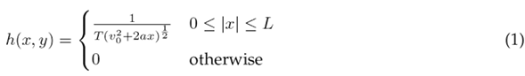
where a, v o , x, and T are the values of the uniform acceleration, the initial velocity, the displacement, and the exposure time interval, respectively. Fig. 1a illustrates the PSF for constant velocity, and Fig. 1b does so for constant acceleration. Notice that Eq. (1) becomes Eq. (2) when a = 0, which corresponds to a uniform velocity. The product Tv o is equal to L, the blur’s length. Additionally, the Fourier Transform of both is depicted in Figs. 1c and 1d, respectively. Moreover, note that a constant acceleration causes a smear in the Fourier Transform of the PSF, which complicates parameter extraction.
Figure 1 PSF for (a) uniform velocity and (b) uniformly accelerated motion. (c) Fourier transform of the PSF in (a) and (d) Fourier transform of (b). These are only illustrative examples
We cannot infer where the camera is moving towards using the PSF shown in Eq. (1). When the capture system is moving at a constant velocity, the PSF is symmetrical with respect to the y-axis. It does not provide any clue as to whether the motion is from right to left or from left to right. A particular situation arises when the system is accelerated. When this happens, the initial velocity is different from the final one, so the PSF curve is not symmetrical. There are two cases: if the initial velocity is lower than the final one (positive acceleration), the PSF curve is higher on the left side. On the contrary, when the final velocity is lower than the initial one (negative acceleration), the function is higher on the right. Thus, the PSF does not allow determining the motion’s direction.
When the camera is not operating horizontally, the angle of motion can be measured regardless of the velocity and the acceleration if the motion blur is long enough.
In some cases, such as velocity estimation, the PSF height
 is not explicitly required. Velocity 0 can be calculated using the blur length L and the exposure time T , although height is also related to the initial velocity (Fig. 1a). On the other hand, acceleration can be calculated using Eq. (3). The blur length L in pixels can be obtained from the inverse Fourier transform of Fig. 1d. However, to estimate the acceleration a, information about the change in velocity
 is also needed. Although v
0 and v
f
are, at first glance, inferable from the PSF (Fig. 1b), they do not correspond to the values obtained, since the extracted PSF is also altered by the exposure time, the brightness, the contrast, the noise, and the image’s frequency content, among other aspects.
is also needed. Although v
0 and v
f
are, at first glance, inferable from the PSF (Fig. 1b), they do not correspond to the values obtained, since the extracted PSF is also altered by the exposure time, the brightness, the contrast, the noise, and the image’s frequency content, among other aspects.
Some authors have concluded that uniform acceleration causes less degradation to the image than uniform velocity (22-24). Partly for this reason, it is more difficult to estimate acceleration than velocity from a single motionblurred image. As an example, Fig. 2 depicts the difference between constant velocity and accelerated motion. Most frequency methods use the zero crossings of the collapsed Fourier transform of the motion-blurred image to estimate the blur length 25)-(28. The zero crossing values are inversely related to the PSF length. When a uniformly accelerated blur degrades the image, its Fourier transform valleys move away from the zero-crossing line axis.
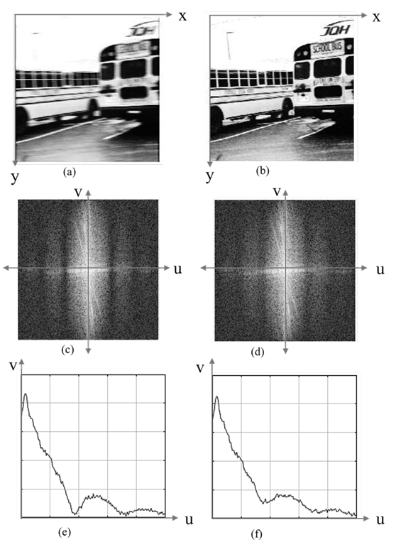
Figure 2 Differences between a degraded image with a uniform and a uniformly accelerated motion blur. (a) Invariant motion-blurred image related to constant velocity. Here, the blur is more visible to the naked eye. (b) Invariant motion-blurred image related to constant acceleration. Here, the blur is lower. (c) Modulation transfer function of (a). (d) Modulation transfer function of (b). (e) Collapsed MTF on the u-axis of (c). (f) Collapsed MTF on the u-axis of (d)
Kinematic quantities using vision-based approaches
The PSF has an essential role in image formation theory. All-optical systems have a characteristic PSF, which intrinsically describes the degradation process of the image during its formation. Therefore, the PSF can include information about kinematic quantities such as motion, velocity, and acceleration over the exposure time.
Its nature can help to classify blur as optical, mechanical, and medium-induced blur 19. This document only considers the mechanical blur that happens when the objects and the camera capturing the image move during the exposure time of the light sensors 20.
Motion blur approaches
20 and 29 introduced a way to calculate the speed of vehicles from a single motion-blurred picture, with the aim of supporting transit authorities. Their proposal used the geometry of the scene, the camera parameters, and the blur length. These authors stated that their method’s error was less than 10 % when applied in real speed detection scenarios.
30 suggested an approach to measure the speed of a vehicle using motion blur analysis which involves inspecting the speedometer of automotive vehicles. Speed was calculated by analyzing the characteristics and regularities in a single blurred image of a simulated road surface. The authors reported errors of less than 10 %. Moreover, there is some research on speed estimation from actual motion-blurred, as is the case of 31), (32, and 33).
34 used code exposure for the accurate reconstruction of motion-blurred images. They proposed statistical blur calculations to obtain precise motion measurements of constant velocity, constant acceleration, and harmonic rotation in actual pictures. For their experiments, they took pictures of a toy car that slid freely on a tilted track only under the influence of gravity. Alternatively, they generated harmonic rotation by using a pendulum-like system. The authors set the camera at the same angle as the tilted platform in order to make the blur almost horizontal in the captured image. They validated their method by measuring the quality of de-blurred images. These authors only estimated motion because their work was mainly focused on image restoration, which does not require a precise reconstruction of the point spread function to improve the image. Their study was based on 35.
36), (37, and 38 introduced a method for estimating the velocity of a vehicle using a camera moving in the opposite direction to generate blur. They argued that the inclination of the motion blur pattern line in a single image was inherently linked to the velocity of the vehicle and the modulation speed. They also denoted that the inclination level could be calculated by employing line detection techniques such as the Hough transform or the Gabor filter. They estimated that the absolute velocity error was below 2,13 km/h and concluded that their method was independent of the exposure time. Lastly, they inferred that their proposal could be used for vehicular technology.
39introduced a defocus correction procedure to obtain the velocity of particles from a single-frame and singleexposure image (SFSEI). They based their proposal on the changes in focus, size, and shape of particles, both close and distant, captured in a blurred snapshot. This method was confirmed in a free-falling particle experiment.
40presented a method to determine the position and calculate the velocity of an object by locating the blur’s initial and final position. The researchers noticed that, under constant illumination, the motion’s start and end could not be determined. To solve this issue, they used modulated illumination, i.e., red light at the beginning and blue light at the end, in order to tag the blurred image. They reported that their method had not yet been implemented in real conditions.
The work by 42 and 43 introduced a technique to calculate velocity from a single linear motion-blurred picture. The discrete cosine transform was used to extract the PSF of the actual motion-blurred images as a basis to measure the blue extent L and the angle. This was done in combination with the exposure time T .
44 proposed a novel approach involving adversarial blur attack against visual object tracking algorithms. Rather than adding imperceptible noise, they actively synthesized natural motion blur on video frames in order to mislead state-of-the-art trackers. The attack was performed by tuning two sets of parameters controlling the motion pattern and light accumulation process that generate realistic motion blur. An optimization-based attack iteratively solved an adversarial objective function to find the blurring parameters. A one-step attack predicted the parameters using a trained neural network. Experiments on four tracking benchmarks demonstrated significant performance drops for multiple trackers, showing the threat of adversarial motion blur. The key contributions of this work were introducing adversarial motion blur as a new attack angle and designing optimization and learning-based approaches to craft natural adversarial examples. The limitations included heavy computation loads for the optimization attack and reliance on a specific tracker for training examples. All methods proposed by the authors used video frame sequences instead of a single image, and this attack revealed the brittleness of trackers against common video corruptions, thus motivating the development of robust motion-blur algorithms.
Multi-frame approaches
45 introduced a cell segmentation and competitive survival model (CSS) together with the traditional methods of particle image velocimetry (PIV). They used their algorithm with actual and artificial pictures and made comparisons with other strategies.
3presented a system to estimate the position, velocity, and acceleration of a planar moving robot using a calibrated digital black-and-white camera and light emission diodes as markers. They employed a multi-frame approach that made use of the Kalman filter to calculate velocity and acceleration. These authors stated that the blur motion should be limited, so that the exposure time was short when compared to the change in the position of the light markers. They concluded that their video approach method is accurate, but they suggested that using a faster CCD sensor would yield better results.
4suggested an acceleration measurement approach using various synchronized video cameras based on videogrammetric reconstructions. Their method located the centroid of visible marks set by the researchers on a shaft run by a shaker. They built a prototype to carry out the proof of concept. They also attached some calibrated accelerometers directly below the target marks in order to obtain ground-truth data to compare with their results. They calculated the second derivative of the videogrammetric position data using the seven-point numerical algorithm to estimate the acceleration. Finally, they provided some overlapped plots aimed at contrasting their results to the accelerometer’s measurements. They concluded that their results were similar to those obtained using accelerometers.
No error was explicitly calculated.
13 proposed a variational method to estimate the acceleration of dynamic systems based on image sequences. They stated that their approach went further than the traditional optical flow methods because they can calculate acceleration. They also pointed out that fluid flow images for calculating acceleration have not been thoroughly studied, even though they are of significant interest. They suggested the use pf acceleration fields and an energy function for their calculations, relying on space-time constraints. When they confronted their results to ground-truth data, they estimated a 7 % average relative error.
Moreover, 46 described a non-invasive method to estimate the pressure distribution in a flow field while employing PIV.
47proposed an approach to measure the speed of a rotating item. They used a pair of cameras to capture a temporal sequence of pictures from coded targets (CTs), which were set on the rotating surface of the object to work as visual marks. This feature matching-based algorithm depends on the motion estimation of contiguous target image pairs. In their experiments, the authors used a rotating fan at 120 rpm and a convolutional neural network (CNN) to identify changes in the position of the CTs during the exposure time. Even though they did not explicitly calculate the speed of the blades, they concluded that their method benefits high-speed object measurement applications. This technique used multiple consecutive images to calculate speed and acceleration.
48introduced a computationally efficient computer vision method to estimate the trunk’s flexion angle, angular speed, and angular acceleration during lifting by extracting simple bounding box features from video frames. Regression models estimated trunk kinematics from these features. The advantages of this approach are computational efficiency, non-intrusiveness, and the potential for practical lifting assessments in the workplace, and its limitations include reliance on simulated training data and lower precision than motion capture methods. This study demonstrated the feasibility of using simple video features to estimate biomechanical quantities related to injury risk, allowing for automated ergonomic evaluation over extended periods.
In their review, 49 covered deep learning methods for the estimation of fluid velocity fields, including fluid motion estimation from particle images and velocity field super-resolution reconstruction. Supervised and unsupervised convolutional neural network approaches have shown excellent performance in estimating fluid motion from particle image pairs. GAN and physics-informed neural network methods have also shown potential for the high-resolution reconstruction of velocity fields. The key advantage of deep learning is the ability to learn feature representations directly from data, thus surpassing traditional methods. Limitations included the need for extensive training datasets and difficulties in incorporating physical knowledge. All reviewed methods used video sequences or image pairs for estimation. Overall, this review demonstrated that computer vision and deep learning hold great potential for estimating kinematic quantities in fluid flow and human biomechanics applications, with anticipated growth in the future integration of these methods.
Further reading about PIV acceleration measurement can be found in 50 and 51, and other multi-frame video strategies for velocity are shown in 52), (53), and 54.
Works related to machine learning
55 used support vector machines (SVM) regression to forecast water flow velocity. Even though they asserted that their approach was not fully successful - as expected -, it was promising and useful for future research.
56 suggested a method for estimating the velocity profile of small streams by using robust machine learning algorithms such as artificial neural networks (ANNs), SVMs, and k-nearest neighbor algorithms (k-NN), with the latter outperforming the others in the results.
57 introduced a machine learning approach based on a CNN model to estimate velocity fields using PIV with missing regions. These authors also argued that, despite recent advances, no studies have focused on machine learning applications using this approach. They used artificial images generated with a direct numerical simulation, concluding that it is possible to estimate the velocity fields with less than 10 % error.
The work by 58 should be highlighted, as they suggested a method to assess structural damage by estimating acceleration at multiple points via a traditional sensor approach. Alternatively, they interpreted the results using the supervised machine learning algorithm called random forest.
As mentioned above, some remarkable studies have been carried out to estimate velocity and acceleration from multi-frame and multi-camera methods. However, we did not find any strategy based on motion-blurred images for measuring acceleration.
Works related to deep learning
Deep learning is a technique derived from neural networks that has recently supported instrumentation and measurement. In the scientific literature, it can already be found in combination with traditional instrumentation, such as light detection and ranging (LiDAR) 59), radars 60, and PIV 61, 62, in order to estimate the velocity of objects and particles. However, we found no evidence of similar works using deep learning and a single motion-blurred image.
Estimating kinematic quantities from a single image is a challenging yet potentially beneficial issue. A moving system, such as a vehicle, a robot, or a drone, can use motion-blurred images to estimate these parameters without the need for bulkier, heavier, and more expensive devices. Moreover, processing one image is often easier than processing a video sequence.
The contributions of this study are as follows:
The construction and metrological calibration of an electromechanical incline slider to generate different acceleration values.
The development of a dataset with 125 invariant, uniformly accelerated motion-blurred images in a controlled environment.
The comparison of some machine learning techniques against deep learning for acceleration estimation.
A proposal for the estimation of acceleration from a real single invariant, uniformly accelerated motion-blurred image
The remainder of this paper is organized as follows. Section 2 introduces our proposal for acceleration estimation using machine learning and the PSF as a source of characteristic feature patterns. Section 3 presents the experimental setup and the testing carried out. Section 4 outlines the results obtained in the experiments by comparing different regression approaches (including deep learning) and their metrics. Section 4 contrasts the results with those of previous authors and discusses the limitations and benefits of the method. Finally, Section 5 presents the conclusions of this work.
This paper is a product of and reuses, with due authorization, content from the PhD thesis and research project entitled “A contribution to the estimation of kinematic quantities from linear motion-blurred images” cited in 43.
Proposed measurement method
An image system is modeled as the convolution of the PSF with the blur-free image. This does not allow for the use of linear filtering approaches to extract the PSF. Alternatively, homomorphic filtering uses nonlinearity transformations, such as logarithmic transformations, to map convolution into a separable linear additive domain (63-66). As a theoretical basis, this research used the homomorphic filtering principle to extract the PSF.
Consider that g(x, y) corresponds to the degraded blur image, i(x, y) is the blur-free image, and h(x, y) represents the degradation kernel (PSF). If noise of any kind is not added and the blur system, it is considered to be linear and stationary, and the process can be described as seen in Eq. (4):

The product ∗ denotes convolution in two dimensions. Additionally, the image convolution from (4) can be also represented as an integral, as shown in Eq. (5):

Considering that Eq (5) deals with finite blur images in space, it is defined in the intervals x 2 ≤ x ′ ≤ x 1 and y 2 ≤ y ′ ≤ y 1. It should be noted that the convolution interval must be larger than the PSF interval of the blur.
Now, the discrete Fourier transform (DFT) is applied to both sides of Eq. (4) to obtain Eq. (6), which represents a point-wise multiplication in frequency domain instead of a convolution in space.

G(u, v), as shown in (6), is a complex value, so it can also be written in polar coordinates using magnitude and angle, as shown in Eq. (7).

This relation can be split into magnitude and phase components, as shown in Eqs. (8) (10), respectively.

Only the log magnitude portion of the complex logarithm of the DFT is used, as shown in Eq. (10).

Although some images can be very different in space, their average frequency is usually very much alike and almost indistinguishable to the naked eye. This allows using the average of Q hypothetical blur-free images I(u, v) k to estimate the prototype clear blur-free image P (u, v) in frequency, as shown in Eq. (11) 65.
in such a way that


Replacing Eq. (13) into Eq. (10), and then solving for |H(u, v)|,

where |H(u, v)| is the modulation transfer function (MTF) of an arbitrary blur, which can be estimated without knowledge of the actual blur-free image using a set of Q reference images to generate a prototype-average log spectrum.
Even though the classical approach for the PSF estimation of an image suggests using statistically close images to generate the prototype average log spectrum, this study used 5 still background images as the clear image in order to estimate the MTF only once for all the experiments. Q = 5 was recommended in 65. Subsequently, the inverse Fourier transform (iDFT ) of H(u, v) is applied to obtain h(x, y), the PSF, as seen in Eq. (15).

Fig. 3 presents the proposed method for acceleration estimation using homomorphic filtering and machine learning regression. In this method, five blur-free images i(x, y) k are taken to the unchangeable background with the camera at rest. This helps reduce the additive noise, subtracting the average of a set of hypothetical blur-free images. Consequently, the MTF is obtained for each of the five images and then averaged, added, and divided by five. This yields a prototype blur-free background log |P |, which is subtracted from the MTF of the motion-blurred image log |G(u, v)| to obtain the output s(u, v). Afterwards, the exponential function is used to remove the logarithm. This allows obtaining the optical Fourier transform H(u, v) of the blurred image, which leads to the PSF h(x, y) in two dimensions via the inverse Fourier transform. As the motion occurs only in the horizontal axis, the actual PSF in one dimension h(x) can be extracted from the central horizontal line of the PSF h(x,y)
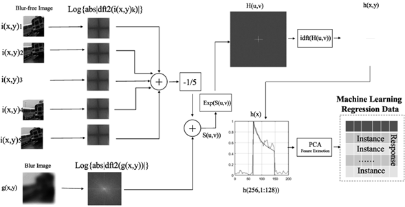
Figure 3 Diagram depicting the process followed to estimate acceleration using homomorphic filtering while applying machine learning. Some blur-free images of the background are needed to separate the PSF for training
Therefore, this research took only the central horizontal row of the inverse Fourier transform, yielding a one-dimension vector containing the characteristic PSF.
If the motion is not horizontal, the one-dimension PSF can also be extracted, but the angle of rotation of the line must be estimated and then rotated. This angle can be calculated using the Radon transform, the Hough transform 42, or principal components analysis (PCA).
Before training, the instances are space-reduced to avoid redundancy using PCA. Finally, a set of uniformly accelerated motion-blurred images with a known acceleration is used for training.
Methodology
The experiments presented in this section were carried out to measure constant acceleration from a linear motion-blurred image by using homomorphic filtering to extract the PSF and machine learning to predict the actual response. First, all parts of the rig setup are introduced, with the purpose of providing a more detailed description of the procedure. Then, an overview of the aforementioned machine learning and deep learning methods is presented, and, finally, the evaluation metrics are described regarding the regression methods evaluated.
Rig setup parts
This section shows the materials and the laboratory equipment needed for the experiments, some of which were specifically constructed within the framework of this study.
Slider
A 185-cm-long aluminum slider constructed for previous speed experiments was used 42, which was slightly modified for our study. Fig. 5 shows the physical layout parts modeled in order to validate the proposed method. Five preset posters were used as a background scene (Fig. 4). Additionally, the camera was placed in parallel to and 171 cm away from the rig. An inclinometer was also installed on the camera. A constant acceleration was achieved by raising an end of the platform to one of the five possible preset angles (A1, A2, A4, A5, and A7) listed in Table I. Sliding occurred evenly and only under the force of gravity. Fig. 6 presents the rig setup used to carry out the experiments. More information about its construction and calibration can be found in 67.
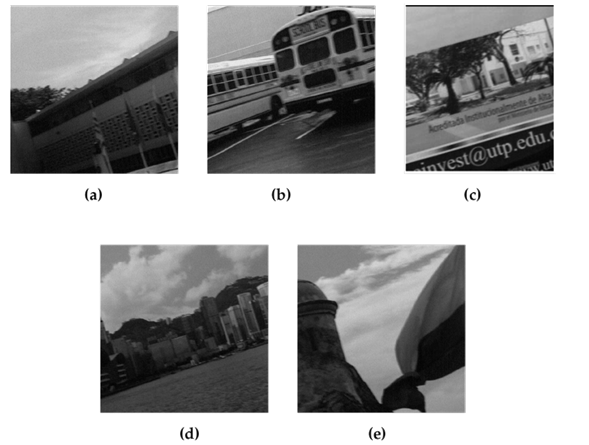
Figure 4 Color version of some accelerated motion-blurred images. The degradation is almost imperceptible by visual inspection
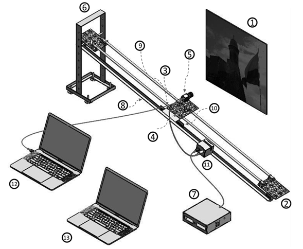
Figure 5 Setup parts and their location. Background pattern poster (1), leveling rubber feet (2), digital pitch gauge-inclinometer (3), camera sliding carriage platform (4), camera (5), lifting base (6), controller (7), oiled stainless steel rods (8), low-friction linear bearings (9), laser-cut toothed steel sheet (10), camera trigger (11), image capture computer (12), and data analysis computer (13)
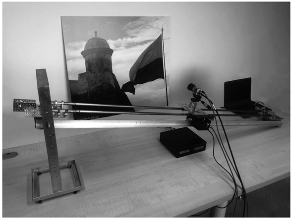
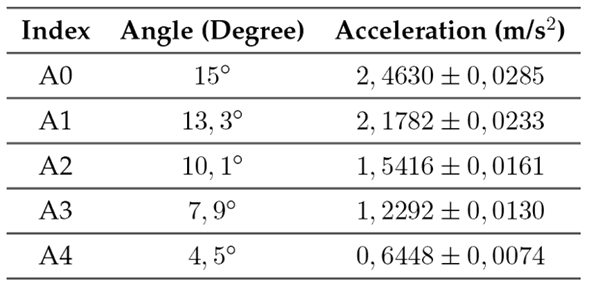
Image analysis system
Motion-blurred image capture and processing were performed on a 64-bit desktop computer with a Core I3 processor and 2GB RAM. Additionally, a 64-bit laptop computer with an AMD A3 processor and 2GB RAM was used for analyzing the acceleration data from the controller system. Both computers used Windows 7 and were running MATLAB 2017b.
Images
Our experiments were carried out in a controlled environment. A scientific digital camera (Basler acA2000-165um USB 3.0) 68 was used to take the pictures. In addition, the artificial white light from the led panel lamps was about 255 Lux, the distance to pattern poster was set at 171 cm, the maximum exposure time of the camera was 100 ms, the slider acceleration was between 0,6 and 2,40 m/s2, and the aperture of the lens diaphragm 69 was F/4.
Blurred images of five different pattern posters were taken (Fig. 4). Afterwards, the captured digital images were clipped and converted to grayscale 70. These experiments considered the angle of motion at zero degrees. Although the camera slid on an inclined plane, the motion blur was horizontal with respect to the camera angle. The background scene posters were not rotated, so, at the naked eye, they looked crooked. Fig. 5 shows each of the elements described.
PCA feature extraction
Feature extraction is a relevant topic in signal processing, mostly due to the high dimensionality of data and their redundancy 71. PCA is a classical and widely accepted statistical approach for feature extraction in pattern recognition and computer vision 72. In this study, PCA feature extraction was used to reduce redundant data from the extracted PSF. The multidimensional space was transformed from 125 to 76 characteristics.
Machine learning regression
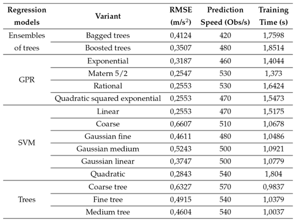
Five different approaches were used to predict the acceleration from the PSF data of actual motion-blurred images. Tree ensembles, Gaussian processes (GPR), and linear, SVM, and tree regression and their variations were evaluated, as presented in Table II.
Table II Machine learning results obtained using tree ensembles, GPR, and linear, SVM, and tree regression
Regression model assessment
The metrics applied to assess the regressions were the root mean square error (RMSE), the prediction speed in observations per second, and the training time in seconds.
Experimental results
Five pictures were taken at each of the five preset accelerations. Additionally, five background scene posters were used, for a total of 125 motion-blurred images.
Although the acceleration values were almost always the same as in Table I, the error was estimated individually using the electromechanical instrument and our vision-based acceleration values.
Instrument calibration
The uniformly accelerated motion system involved an Arduino Nano microcontroller, which was responsible for measuring the time it took to block each tooth of the steel sheet. Its operation consisted of allowing the camera carriage platform on the steel rods to slide at five different angles, yielding different accelerations depending on the height. The angles and their accelerations are shown in Table I.
Calibration was performed by measuring the acceleration with both the controller system and the Phywe Cobra4 Sensor-Unit 3D-Acceleration standard instrument (±2 g and a resolution of 0,001 g), using the Cobra4 wireless link to transmit the acceleration data 73. The combined uncertainty and the sensitivity coefficients were evaluated to estimate the total expanded uncertainty according to guidelines regarding the expression of uncertainty in measurement 74), (75. See 67 for more detailed information about the calibration process.
Data acquisition results - Machine learning
Five folds were used to validate all of the proposed regression models. Table IIshows the results for the basic regression models and their variants. Note that, even though only five major approaches were assessed, each one had a subset of variants, for a total of 19. The best RMSE results were reported by GPR (Matern 5/2), linear regression, and SVM (quadratic) regression, with 0,2547, 0,2553, and 0,2843 m/s2, respectively. GPR (Matern 5/2), linear regression, and SVM (quadratic) regression reported values of 530, 470, and 540 obs/s, respectively. Finally, the fastest training time corresponded to GPR (Matern 5/2), with 1,373 s. See Table II for more details.
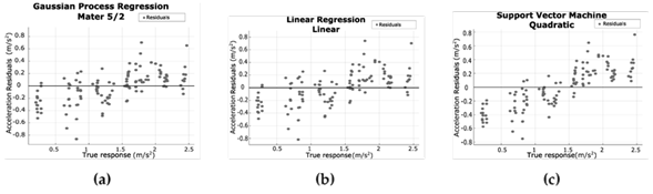
Moreover, predicted vs. actual and residuals plots were employed for the best three RMSE results. The residuals plots for GPR (Matern 5/2), linear regression, and SVM (quadratic) regression (Figs. 8a, 8b, and 8c, respectively) showed that the acceleration residuals tend to change their sign from negative to positive when the acceleration is higher than 1,4 m/s2. Furthermore, the acceleration residuals are smaller in all cases when the acceleration is higher than 1,0 m/s2. This makes GPR (Matern 5/2) more suitable for real-time applications. In summary, the plots for GPR (Fig. 8a) and linear regression (Fig. 7) are almost identical.
As expected, decision trees showed the worst results since they tend to fail when training data is limited.
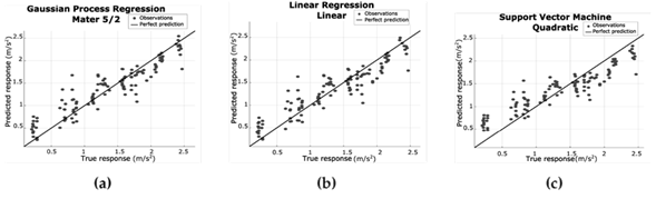
Figure 7 Predicted vs. actual plots for (a) Matern 5/2 regression, (b) Linear regression, and (c) SVM regression
Data acquisition results - Deep learning
Deep learning techniques have some advantages, such as the automatic extraction of features. In addition, input images can be used without any prior processing beyond the geometric transformations of the training images when expanding the dataset becomes necessary. Therefore, in this part of the experimentation process, homomorphic mapping was not used as a source of features for the regression.
The executed algorithms were coded in MATLAB R2020b, using the Deep Network Designer toolbox. It is crucial to emphasize that the learning algorithm corresponds to a regression instead of a classification process, which allows generating response values outside the training data.
As mentioned earlier, 125 training images were used, which were 512 x 512 x 3 pixels in size. However, the pre-trained networks required different dimensions. Therefore, the pixel size of the images was set at 224 x 224 x 3 for GoogleNet and VGG-16, at 227 x 270 x 3 for AlexNet, and at 299 x 299 x 3 for Inception ResNet-v2.
The performance of a CNN depends mainly on hyperparameters such as the learning rate, the mini-batch size, the number of epochs, the number of iterations, and the solver algorithm. For a good performance, a determining factor is the pre-trained model, which typically uses hundreds or thousands of images. Therefore, in our study, it was necessary to extend the image dataset by performing rotations and reflections to obtain 750 images. The image size scale was not changed, as it implicitly includes the blur length attributes.
The dataset was divided as follows: 80 % for training, 10 % for validation, and 10 % for testing. Thus, the 750 images were divided into 600 training images, 75 validation images, and 75 testing images. All of them were randomly selected from the dataset.
As can be seen in Table III, AlexNet offered the shortest training and prediction times while using the GTX1650 and the GTX1050 GPUs. Regarding the RMSE, the lowest value (0,4639 m/s2) was obtained using Inception ResNet v2. However, this is far from what was achieved using homomorphic mapping, which showed a smaller RMSE (0,2547 m/s2).
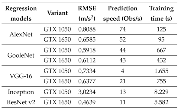
It should be noted that only GPUs were used with the deep learning algorithms and CPUs with the machine learning algorithms.
Discussion
Even though there are some studies on estimating speed using vision-based measurement (VBM), to the best of our knowledge, only a few deal with acceleration. Likewise, there is no evidence of studies that estimate acceleration from a motion-blurred image.
Some approaches have been introduced to measure acceleration, and all of them require at least two consecutive frames 45), (46), (76, while others also use high-speed or multiple cameras 4), (77, thus making make classical approaches more expensive and bulkier.
This field of research has great potential across various applications, including forensic sciences, particle physics, and autonomous drones. The proposed technique can extract essential motion parameters from a single image, simplifying processes that traditionally rely on multiple video frames or complex sensor configurations. Consequently, it reduces the complexities associated with runtime and computation, resulting in substantial savings regarding storage space and energy consumption. This efficiency makes it an environmentally sustainable and cost-effective approach, underscoring its importance.
The acquisition of blurred images relies on the adjustment of camera settings, particularly the exposure time relative to the scene’s motion. While creating motion blur is relatively straightforward in general photography, achieving controlled motion blur in scientific or forensic contexts often requires specific conditions. Moreover, analyzing the variables, conditions, or parameters involved in obtaining motion blur becomes more intricate when the subject or object in motion is not the camera itself. In such scenarios, both the camera and the subject’s movements affect the resulting blur, necessitating the application of specialized methodologies. The attributes of a camera employed to capture motion blur data are not rigidly prescribed, but several critical features contribute to its effectiveness. These encompass adjustable exposure settings, sensor sensitivity, image stabilization capabilities, and the camera’s lens and sensor quality. These attributes significantly influence the quality and reliability of the analysis. Consequently, the selected camera and its settings emerge as a pivotal consideration, with a substantial influence over the outcomes of motion blur analysis in diverse applications.
This alternative blur-based method has benefits. Motion blur is a usual and undesirable degradation, but it is possible to take advantage of it, as it allows for acceleration estimations. In addition, this approach can be implemented with low-cost cameras, instead of high-speed multi-frame video equipment, which is more expensive.
Likewise, the proposed method has some limitations. One is that it needs a set of blur-free images as reference for training. However, in some cases, this is easy to obtain from the background. For example, a drone can obtain the prototype images from an initial image (a prototype with no motion blur) of a crop and then fly over it while estimating the acceleration. Noise is another limitation of this proposal: when the noise is dominant, the extraction of the PSF can fail along with the estimation. Finally, the space-invariant model introduced in this study assumes that the exposure time is relatively short, and the length from the rig setup to the camera is fixed to ensure invariant blur on all images.
Conclusions
With some degree of accuracy, the machine learning models successfully estimate relative acceleration from a single motion-blurred image, using homomorphic filtering to extract the features of the PSF, which depends on the initial velocity, the acceleration, and the exposure time, as shown in Eq. (1).
The proposed method is a valid alternative to estimate acceleration with invariant motion blur. The best machine learning methods were GPR (Matern 5/2) and linear regression, with RMSE values of 0,2547 and 0,2553 m/s2, respectively. These methods were able to perform 530 and 470 obs/s, respectively. Finally, the best results were obtained when the acceleration was above 1,0 m/s2. This makes machine learning an alternative approach that can be used in real-time applications for estimating acceleration when motion blur is invariant, and noise is not dominant

