


 English (pdf)
 Article in xml format
 Article references
 Send this article by e-mail
 Cited by SciELO
  Cited by Google
  Similars in
SciELO
Similars in
SciELO  Similars in Google
 Permalink
1. Introduction
Special Economic Zones (SEZs) are delimited geographic areas contained within a country's national boundaries, with natural and logistical advantages suitable for high productivity. SEZs provide an exceptional business environment to attract investment, develop international trade, generate quality jobs, as well as offering fiscal and labor benefits, a world-class infrastructure and support programs (human capital, financing, and innovation). SEZs promote the economic activity within the zone and the industrial zones that focus mainly on specific economic activities [1].
The World Bank considers that the concept of an SEZ includes a wide variety of types of economic zone. Among the most important are Free Trade Zones (FTZs) which re-export goods enjoying certain customs advantages, and Export Processing Zones (EPZs), which promote economic growth by attracting foreign investment and producing exports [2,3].According to Zeng [4], in the last three decades, China has been an example for other countries in the creation of SEZs, because these have contributed significantly to the generation of employment, exports, gross domestic product and attraction of foreign investment.
In 1980, the first four SEZs of China were created: Shenzhen, Zhuai, and Shantou belong to Guangdong Province and Xiamen belongs to Fujian Province. These two provinces are strategically located in coastal areas close to Hong Kong, Macao, and Taiwan. Of all these zones, Shenzhen is the most developed, probably because of its location at the delta of the Pearl River and immediately north of Hong Kong where capitalist modes of economic growth and management have flourished [5]. Several studies are still assessing the great economic achievement of this region, in order to replicate it [6].
The success of SEZs inside China has inspired other countries, such as Honduras, Taiwan, South Korea, Madagascar, India, El Salvador and Bangladesh, to create their own. This has provided multiple benefits, such as employment generation, export growth and diversification, government revenue and technology transfer [1,7-10]. For instance, India is one of the many countries where, thanks to the establishment of SEZs, the jewelry and electronics industry has grown rapidly and this has contributed to creating quality jobs [11,12]. Through a three-sector Harris-Todaro type model it has been established that agriculture and SEZs can grow at the same time if the government provides support for projects that benefit and boost land efficiency [13].
The main contribution of this paper is to propose a tool for delineating SEZs based on mathematical modeling. Our method is applied in a case study of the Isthmus of Tehuantepec, Mexico.
2. SEZs and mathematical modeling
For a decision maker, designing an SEZ is not an easy task, mainly due to two reasons: defining the spatial unit to use (province, state, town, etc.), and determining its area of influence. Mathematical tools, in particular, Integer Linear Programming (ILP), have been used to solve several complex real-life problems where the decision maker does not find it easy to make a decision.
The problem of the delineation of SEZs is similar to the territory design problem (TDP), where small geographic basic units (municipalities) are grouped into larger geographic clusters called territories (economic zones), which are acceptable or optimal according to the relevant planning criteria [14]. The TDP has several applications in political districting [15-20], sales territory design [14,21-23], agricultural zones [24,25] and public services [26]. Some surveys of the methods and algorithms used in the TDP can be found in [27-29] for districting problems; in [26] for sales districting and; in [30] for political districting.
The originality of the present paper lies in the way to treat the delineation of SEZs. To the best of our knowledge, there are no studies using an Integer Linear Programming approach to delimiting these zones and their areas of influence. In this article, we propose two mathematical formulations to delineate SEZs and their areas of influence. The first one is based on the assignment problem and, the second one on the facility location problem.
3. Methodology
Some specific characteristics that have been of great importance when creating an SEZ are a) the internal characteristics of the zone, b) its relative location and, c) its interactions with areas of intense commercial activity [4]. Taking into account these characteristics we propose a new method to delineate SEZs by using ILP. We present two mathematical formulations. In the first one, we consider the time and distance between the municipalities, their popula-tion, any extreme poverty, and the infrastructure of the region. A particularity of this model is that some munici-palities are fixed previously as the center of each economic zone. In the second model, the same considerations are taken, but the center of each SEZ is optimally chosen by the model considering a set of potential sites, given previously, where the center of each SEZ can be determined.
3.1. Model A
In this model, the minimum number of SEZs is previously computed according to the population density and the restrictions on population imposed by the government. Then, the center for each SEZ is established a priori considering the potential of each municipality. Finally, the model selects the best way of assigning municipalities to an SEZ.
To formalize this problem, let I be the set of municipalities where I={1,…,m}, and let J be the set of SEZs where J={1,…,n} computed by Eq. (1), where; p i is the population of municipality i, and UP is the maximum population allowed in an SEZ. Therefore, the minimum number of zones is initially given by the following equation:

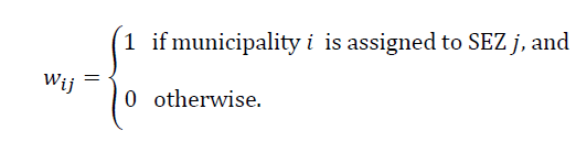
The objective is to minimize the distance Dij from a municipality i to an SEZ j. The model must satisfy the bounds of minimum and maximum population (LP and UP, respectively) previously established. The decision variables for this formulation are:

The resulting mathematical model is:

subject to:


The objective function is represented by (2), where the total distance between municipalities and SEZs is minimized. Constraints (3) ensure that each municipality is assigned to only one economic zone. Constraints (4) and (5) ensure that the population for each economic zone must satisfy the local specifications. Finally, in (6) the nature of the variables is declared.
Version 2 of this formulation minimizes the time instead of the distance. Replacing the objective function (2) we have

where T ij is the travel time from municipality i to potential SEZ j.
An important reason to consider the travel time instead of the distance is that often the available infrastructure, official speed limits, historical traffic speed data, and others, have shown that the distance and travel time are not proportional; in some cases, the travel time can be bigger in shorter distances than in larger distances. Therefore, it is very important to consider the time.
3.2. Model B
This model is based on the facility location problem, which has practical importance in problems where the objective is to choose the location of facilities, such as industrial plants or warehouses, in order to minimize the costs or maximize the profit of satisfying the demand for some commodity (see [31]).
For this model the same parameters are considered as in model A. However, in this case, the selection of each center of an SEZ is chosen by the model instead of being fixed previously. To formalize this, we consider a set of municipalities I={1,…,m} each one with a specific population p i , and a set of potential sites J={1,…,ZONES} where the center of the economic zone can be established. In this case, the potential municipalities in the region define the number of zones, denoted by ZONES, which differs from model A to model B. The distance from municipality i to potential site j is denoted by D ij . The variables for the integer linear programming formulation are:

The mathematical formulation is:

subject to:


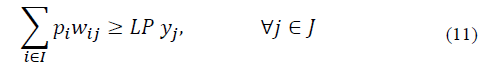


In the objective function (8) the aim is to minimize the total distance between the municipalities and the SEZs. Constraints (9) ensure that each municipality is assigned to only one economic zone, which means a municipality cannot be in two economic zones simultaneously. Constraints (10) and (11) ensure that the population for each SEZ must be satisfactory if it is selected. Constraints (12) ensure that a municipality is going to be assigned to a special economic zone only if it is selected. Constraint (13) limits the number of special economic zones with the minimum number required according to Eq. (1). Finally, in (14) and (15) the nature of the variables is declared.
As in model A, version 2 of this formulation consists in considering the time instead of distance as in (8), and then we have:

3.3. Case study: Special Economic Zones in Mexico
The area of interest for the creation of these SEZs is located in the region of the Isthmus of Tehuantepec in Mexico that includes three states: Veracruz, Oaxaca, and Chiapas (see Fig. 1). This area is considered as a way of transisthmian communication between the Atlantic Ocean and the Pacific Oceans, which impacts on the transportation of goods destined for national and international markets.

Data obtained from the Mexican National Institute of Statistics and Geography (INEGI).
Table 1 shows the municipalities of each state that will be considered when creating the SEZs. The first eighteen municipalities belong to the state of Veracruz and the rest belong to the state of Oaxaca. The first and fourth columns show the ID, the second and fifth columns show the names, and the third and sixth columns show the population for each municipality.
Table 1 Population for each municipality of the Isthmus of Tehuantepec, Mexico.

Source: The Authors.
According to the Mexican Federal Law for the creation of SEZs, these will be established with the aim of boosting through investments the economic growth of the country's regions. They must meet the following requirements:
a) They must be located among the ten states with the highest incidence of extreme poverty.
b) These zones should be established in geographic areas that have a strategic hub with access to large infrastructures such as airports, railways, ports and inter-oceanic highways in order to increase productivity.
c) Each SEZ can be integrated with at least one municipality. Each zone must have a population between 50000 and 500000 inhabitants.
Oaxaca has the second highest incidence of extreme poverty of the states of Mexico, while Veracruz is in sixth place; therefore, the first requirement mentioned above is fulfilled. The objective of creating SEZs in these two states is to exploit their strategic location.
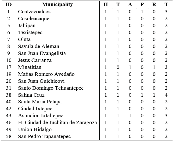
Table 2 shows the infrastructure of the potential munici-palities that are candidates to be the center of an SEZ. The first and second columns indicatae the municipality; the third to seventh columns show the available infrastructure (a ‘1’ means the municipality has a highway (H), train (T), airport (A), port (P) or refinery (R)). The last column shows the total number of elements (T).
4. Results
Experimental results based on real data of the Isthmus of Tehuantepec, México, validate the method and enable a graphical visualization of the solution. In this section, the integer programming formulations for the SEZ problem are validated. The mathematical models were solved using CPLEX version 12.7.0.1 executed on a workstation equipped with 64 GB of RAM and 8 Intel(R) Xeon(R) E5-2609 v4 Processors @ 1.7 GHz.
4.1. Model A
For this model, we first compute the minimum number of SEZs required for partitioning the region of the isthmus using Eq. (1). In this case, the minimum number of zones was equal to 4.
Then, we generate 136 instances considering combinations of 4 municipalities using the potential municipalities given in Table 2.
Taking into account the port infrastructure of Coatzacoalcos (1) and Salina Cruz (38), they were fixed as the centers of the first two SEZs. The number between parentheses means the ID given in Table 2. The other two centers of SEZs were combined with the other potential municipalities, i.e., Cosoleacaque (2) and Jaltipan (5), Cosoleacaque (2) and Texistepec (6), Cosoleacaque (2) and Oluta (7), and so on to Cosoleacaque (2) and San Pedro Tapanatepec (58). The same was done with the rest of the potential municipalities.
Tables 3 and 4 show the experimental results for the 136 instances considering the version 1 of model A (distance). The first and ninth columns present the IDs of the instance; the second to fifth and tenth to thirtieth columns present the IDs of the municipalities established as a center of an SEZ (see Table 1); the sixth and fourteenth columns are the distance in km obtained by the model; the seventh and fiftieth columns are the travel time in minutes computed with Table A1 and using the solution obtained by the model; the eighth and last columns are the solution time in seconds taken by the solver.

Tables 5 and 6 are very similar to Tables 3 and 4, just that these results are from version 2 of model A (time). The travel time in minutes is the solution of the model, and the distance is computed with a table similar to A1 but considering distance instead of time.


Fig. 2 presents the solution for the 136 instances comparing the distance for both versions of model A. The distance for the first version (circles) is the value of the objective function (column distance of Tables 3 and 4). The distance for the second version (rectangles) is the computed value considering the solution obtained by the model (column distance of Tables 5 and 6). The X-axis represents the instance number and the Y-axis is the value in km of the objective function. In this case, 11.76% of the instances have the same value for both versions while 88.24% have a smaller value in version 1. Note that in no instance does version 2 wins. This behavior is normal because the priority of version 1 is minimizing the distance instead of the time.

Source: The Authors.
Figure 2 Solutions for the 136 instances comparing the distance in both versions of model A.
Fig. 3 shows the solution for the 136 instances comparing the travel time for both versions of model A. The travel time for the first version (circles) is the computed value using the solution of the model in joint with Table 8 (column travel time of Tables 3 and 4). The time for the second version (rectangles) corresponds to the value of the objective function (column travel time of Tables 5 and 6). The X-axis represents the instance number and the Y-axis is the value in minutes of the objective function. As in version 1, 11.76% of the instances have the same value for both versions of the model, while 88.24% of the instances have a smaller value in version 2. Note that in no instance does version 1 wins. This behavior is normal because the priority of the version 2 is minimizing the time.

Source: The Authors.
Figure 3 Solutions for the 136 instances comparing the travel time in both versions of model A.
Fig. 4 shows the configuration for version 1 of model A. The left side is the instance with the least distance, which takes Coatzacoalcos, Salina Cruz, Jaltipan, and H. Ciudad de Juchitan de Zaragoza as the centers of the SEZs. The right side is the instance with the greatest distance, which takes Coatzacoalcos, Salina Cruz, San Pedro Tapanatepec, and Santo Domingo Tehuantepec as the centers of the SEZs.

Source: The Authors.
Figure 4 Configuations of SEZs minimizing the distance in version 1 of model A. The left side is the configuration with the least distance, and the right side is the configuration with the greatest distance.
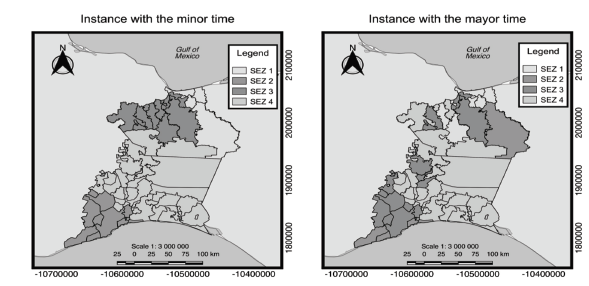
The configuration for version 2 of model A is presented in Fig. 5. The left side is the instance with the smallest time, fixing Coatzacoalcos, Salina Cruz, Cosoleacaque and Ciudad Ixtepec as centers of the SEZs. The right side is the instance with the greatest time fixing, Coatzacoalcos, Salina Cruz, Santo Domingo Tehuantepec and Asuncion Ixtaltepec as the centers of the SEZs.
4.2. Model B
The results for both versions of model B are shown in Table 7. The first column gives the version of the model. From the second to fifth columns are the municipalities which were established as the centers of the SEZs (ID of Table 2). The sixth column represents the objective of the version: distance or time. The seventh column is the value of the objective function in km or minutes. The last column is the time in seconds needed to obtain the optimal solution.

Fig. 6 shows the configuration given by both versions of model B. The left side is the result of version 1, which takes Coatzacoalcos, Jaltipan, Santo Domingo Tehuantepec and Union Hidalgo as the centers of the SEZs. The right side is the result for version 2, which takes Jaltipan, Minatitlan, Matias Romero Avedaño and Santo Domingo Tehuantepec as the centers of the SEZs.

5. Conclusions
In this article, we presented a new approach for the delineation of Special Economic Zones (SEZs). This approach relies on two mathematical models of Integer Linear Programming which consider the federal laws imposed by the government and the natural and logistical characteristics of the region. In the first model, the centers of the SEZs are pre-established according to the minimum number of zones required considering the population and infrastructure of the region. The second model considers the same parameters as the first one, but chooses all the centers of the SEZs. Each model has two versions, the first one minimizes the distance between municipalities and SEZs, and the second one minimizes time.
Experimental results applied to the region of the Isthmus of Tehuantepec, Mexico, validate the method and show several configurations for the design of SEZs, which allows the establishment of negotiations between the municipalities and therefore the support of the local government in the implementation of these zones.
Some extensions of this approach to more complex model such as a bi-objective mathematical formulation are currently under study.


