


 English (pdf)
 Article in xml format
 Article references
 Send this article by e-mail
 Cited by SciELO
  Cited by Google
  Similars in
SciELO
Similars in
SciELO  Similars in Google
 Permalink
1. Introduction
Colombia undertook in the last decade a series of institutional changes in which the State is given greater responsibility for planning the expansion of its natural gas infrastructure, to ensure the supply and minimize the risk of shortages under possible failures. These reforms require a centralized vision of the operation and planning of the system infrastructure, without losing relevance to the current private participation along the supply chain of this fuel.
This study exposes a methodology to simulate the centralized operation of a natural gas transport system based on minimizing costs and satisfying restrictions. For this, the formulation of a typical operational cost equation of the natural gas system aggregate is presented. It includes production, transport, shortage of demand, and the specific conditions for the physical limits of the constituent elements of the network. Subsequently, the mathematical development is shown to transform such equations into a linear and matrix format and to solve these using common optimization software for linear programming available to the general public.
The methodology proposed here is applied to simulate the operation of the Colombian natural gas system between years 2019 and 2035 with the purpose of projecting its operation cost, the flows in its sections, associated rates, and shortage level, as well as the effects that the construction of new infrastructure would have on these variables. This document consists, besides this introduction, of four other sections: the following section presents the equations that define the operating costs and the restrictions of a natural gas transport network. The third section explains the transformation of such equations to a system of linear matrices that can be solved by common linear programming methods; additionally, as an annex, an example is presented using a natural gas network with few elements. The fourth section presents the results of applying the model described to simulate the future operation of the Colombian natural gas transport network to project its typical variables. Finally, the conclusions and other potential uses of this modeling are presented.
2. Formulation of the natural gas system simulation model
The development of natural gas infrastructure requires previous, extensive and meticulous work to ensure its optimal selection among alternatives, as well as the remuneration of the investment and other associated costs [1]. Part of this previous work includes the simulation of the future operation of the new infrastructure and the comparison of alternative operation scenarios.
The simulation work of these systems has included modeling of the mechanical operation of the networks to estimate the maximum flow capacities and pressures, to reduce the energy consumption of compression and other variables [2,3], and minimize investments in new infrastructure [4]. Moreover, also highly demanding computing work is needed in which a solution is not assured by the nature of the equations of fluid mechanics.
The approach used in this study has the following purposes: first, to estimate the economic effects on the end user in relation to the final costs and tariffs that he/she faces; secondly, obtain information on the operation of each of the elements of the network including production, flows, consumption, shortages, among others. Once completed, this would allow comparing alternative infrastructure expansion scenarios concerning their costs and operation.
The model used in this work to simulate a regional or national natural gas transport network is comprised as a system of nodes that represent the supply sources and the largest consumption centers, interconnected through transport lines that would represent gas pipelines, and routes that mobilize compressed or liquefied gas. For the network mentioned above, the following conditions must be met:
The constituent elements of the system operate at their maximum capacity without contingencies that limit their operation.
This modeling has long-term and stable state purposes (t would have units of months or years). Natural gas storage is not considered within the transport network, so the operation and optimization of each period t are independent of the others.
Operating costs refer to the usage and the production tariffs of the different elements of the natural gas transport and supply system. In this sense, they would reflect the investment and operation costs of the same to ensure their adequate remuneration.
The capacities of the elements are exogenously established and commonly known by the owners of these elements through physical tests and simulations of the mechanical operation of their system.
Under the preceding considerations, the equations that characterize the operation of the natural gas transportation network are set forth below. In these, the variables marked with the symbol † are exogenous parameters, i.e. input data for the model. The others are endogenous, established by solvimg the system of equations and restrictions.
2.1. Operational cost equation
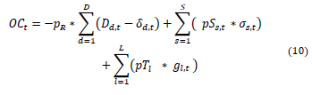
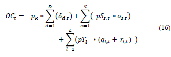
This model is based on minimizing the aggregate cost of natural gas supply, transportation and shortage for each of the periods (t) in a projection horizon, as expressed in the target function (eq 1). This equation could represent flows or volumes, while maintaining the coherence between the variables:
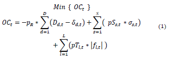
Where:
OC t : Total operational cost of the system in period t;
pR†: Shortage cost (not supply) per flow unit;
D d,t †: Demand required in node d during period t;
δ d,t : Demand supplied (consumption) in node n during the period t. Thus, the magnitude ( D d,t - δ d,t ) is the demand not supplied in node d during period t;
D †: Set of demand nodes;
pS s,t †: Supply cost at the wellhead in the supply node s during period t;
σ s,t : Offer supplied in node s during period t;
S †: Set of offer nodes;
pT l,t †: Transport cost in section (pipe or other) l during period t;
f l.t : Flow in section l during period t;
L †: Set of natural gas transport sections (gas pipelines or other transport lines).
2.2. Operational restriction equations
On the other hand, the restrictions that eq. (1) must meet in each of the periods (t) refer to:
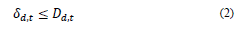
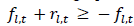
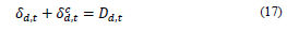
i) Restriction 1 - Consumption limits: The demand supplied in a node is less than or equal to the required demand:
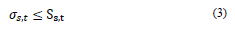
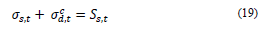
ii) Restriction 2 - Production limits: The production supplied by a node is less than or equal to the maximum production capacity (Ss t), in such a way that:
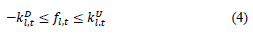
iii) Restriction 3 - Transport limits: The maximum flow transported must be equal to or larger than its inverse maximum transport capacity
 , and equal to or less than its direct maximum transport capacity
 .
.
iv) Restriction 4 - volumetric balance: In all nodes n, the sum of concurrent flows (considering their direction), minus the production plus the demand served is equal to zero. Keep in mind that for this formulation, if the flow (f l,n,t ) enters the node it is assumed as being negative, and if it leaves the node it is assumed as positive:
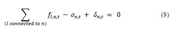
Once this set of equations and restrictions for each period t are solved, the following aspects are established in different elements of the system: the demand served (δ n,t ), the production supplied (σ n,t ), the flow transported (f i,t ), and consequently, the operational cost of the system OC t .
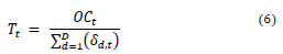
Consequently, the national average rate or tariff (T t ) for period t is defined as:
3. Linear transformation of the equations of the model
As the equations that define the proposed problem have a non-linear character, they must be transformed into a linear format to be able to solve them more easily. Then, these can be structured in the following matrix format detailed below:
Subject to restrictions:
Where:
C T t : is a row vector of exogenous values (input data) that contains the operational costs for each period t.
x T t : is a row vector that contains the operational variables for each period t.
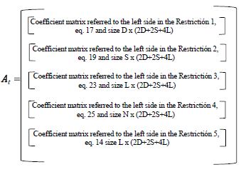
A t : is a matrix of values that represents coefficients of the left side of the restrictions for each period t.
b t : is a vector that contains coefficients on the right side of the restrictions for each month t.
For each of the periods t the matrices C t , x t , A t and b t must be defined. The resolution of the model consists in finding independently, for each of these periods, the optimal vector (x t *) . An example is presented at the end of this document as an annex, applying this model and the matrix ordering, to a natural gas network with few elements.
3.1. Transformation of the target function
The only non-linear term of eq. (1) is
 . To include it into a linear expression, the auxiliary terms g
l,t
, r
l,t
and t
l,t
are introduced according to what is explained below:
. To include it into a linear expression, the auxiliary terms g
l,t
, r
l,t
and t
l,t
are introduced according to what is explained below:

Where in the minimum of the target function:
 ; modifying eq. (1) as follows:
Hereafter, the following two possibilities are considered for g l,t :
(i)
 ; for positive f
l,t
values:
; for positive f
l,t
values:
Implying that:
Using in eq. (11) the eq. (22) set out below, the following equation is formed:
 ; and when it is ordered:

(ii)
 ; for negative f
l,t
values.
; for negative f
l,t
values.
Using eq. (11) the following equation is formed:
and using eq. (22):
Introducing the new term u lt :
Implying that:
Using eq. (13), the eq. (10) is transformed into:

Eliminating the constant and the exogenous terms D d,t and -k D 1 that does not affect minimization, the cost equation becomes:
3.2. Transformation of the restrictions
i) Restriction 1: In eq. (2) the term
 is introduced:
implying that:
ii) Restriction 2: In eq. (3) the term
 is introduced:
implying that:
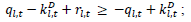
iii) Restriction 3: eq. (4) originates another restriction from the introduction of the terms q
l,t
and
 :
:
Defining a new variable q l,t :

eq. (21) changes to:
 , that when split in two parts: ≤
 and
and
The new variable
 is introduced:
implying that:
iv) Restriction 4: On eq. (5), eq. (22) is introduced generating the following equation:
Where the signs of q
l,n,t
and
 are positive if the flow leaves the node, and negative if it enters it, i.e., consequently with the signs of δ
n,t
and σ
n.t
.
are positive if the flow leaves the node, and negative if it enters it, i.e., consequently with the signs of δ
n,t
and σ
n.t
.
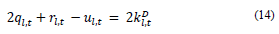
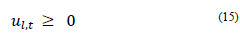
v) Restriction 5: Finally, there is a new restriction oneq. (14):
3.3. Matrix constitution of the typical equations
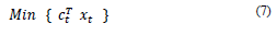
3.3.1. Target function
To structure the target function (linearized in eq. 16) as
 (eq. 7) the following equation is obtained:
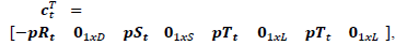 ,
,which is a row vector of dimensions 1 x (2D+2S+4L). Where:
 : row vector of dimensions 1xD that contains the shortage cost (rationing) during period t.
 : zero row vector of dimensions 1xD
 : row vector of dimensions 1xS that contains the supply cost in the supply nodes S during period t.
 : zero row vector of dimensions 1xS
 : row vector of dimensions 1xL that contains the transport cost of sections L during period t.
 : zero row vector of dimensions 1xL.
On the other hand:

which is a row vector of dimensions 1 x (2D + 2S + 4L) with all its components higher or equal to zero, since all the demands of the nodes and productions behave likewise, and as established in Eqs.12, 15, 18, 20, 21, 22 and 24.
Where:
 : row vector of dimensions 1xD that contains the demand supplied in the demand nodes D during period t.
 : row vector of dimensions 1xD that contains the demand not supplied in the demand nodes D during period t.
 : row vector of dimensions 1xS that contains the production in the supply nodes S during period t.
 : row vector of dimensions 1xS that contains the trapped production in the supply nodes S during period t.
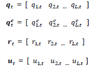
Where
 are row vectors of size 1xL that represent indirectly the flows in transport sections L during period t, as previously defined in numeral 3.2.
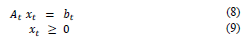
3.3.2. Restrictions
To structure the five restrictions that are already in a linear format (established in numerals 2.2 and 3.2) as
 (eq. 8), the following is detailed:
A t is the matrix that contains the coefficients on the left side of a particular restriction (eq. 17, 19, 23, 25 and 14) that are multiplied by the components of the vecto x t r. Matrix A t has dimensions (D+S+2L+N) x (2D+2S+4L).
Vector b t is consequently composed of five sub-vectors that represent the coefficients on the right side of such restrictions and has dimensions 1 x (D+S+2L+N):

Where:
 : row vector of size 1xD that contains the demand supplied in the demand nodes D during period t.
 : row vector of size 1xS that contains the maximum production in the supply nodes S during period t.

 : row vector of size 1xL that contains the sum of the maximum transport capacities in a direct and opposite direction of sections L of the transport network during period t.
 : row vector of size 1xN that contains the sum of the maximum transport capacities in the opposite direction of the sections that concur in nodes N of the transport network during period t.
 : row vector of size 1xL that contains the maximum transport capacities in the opposite direction in sections L of the transport network during t.
4. Simulated system and results
The previously elaborated model is used to simulate the future operation of the national natural gas supply system in Colombia. The assumptions and main results achieved are presented succinctly below:
4.1. Assumptions used in the simulation
4.1.1. Demand
The demand in the nodal distribution used in this study is methodologically based on the regional and sectorial projection made by Unidad de Planeación Minero Energética UPME [Mining and Energy Planning Agency] [5], divided into 105 nodes that would comprise the national transport network. In the case of Colombia, frequently in the past during the occurrence of the El Niño phenomenon, there were rapid short-term variations in flow contributions to the electricity system which have forced a higher consumption of natural gas for electricity generation.
The preceding implies for the country the need to plan the natural gas supply under conditions of average historical hydrology (Medium Demand), and also considering the possibility that in any year very low hydrology conditions can occur (Demand with the El Niño phenomenon) [6], as shown in Fig. 1. However, for modeling testing purposes, results are presented only for the average demand.
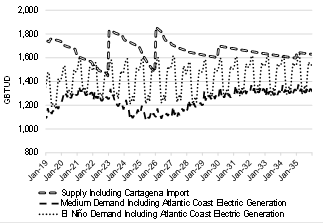
For this demand scenario in the first years, an increase caused by the late entry into operation of the HidroItuango project is foreseen. Subsequently, the demand would grow at decreasingly lower rates until stabilization is achieved in the decade of the 30s.
4.1.2. Wellhead prices and offer
The offer in its nodal distribution that is used in this study is based on the declared production made by the producing companies to Ministerio de Minas y Energía [Ministry of Mines and Energy] [7,8]. Considering that the forward-looking supply will continue to be decreasing due to the decline of the main production fields, since December 2016 the country has arranged an import capacity through the port of Cartagena/Mamonal (400 MMCFD, millions of cubic feet per day). Moreover, it has also planned to dispose of a new import capacity starting from the year 2023 through the port of Buenaventura (400 MMCFD), as well as with other subsequent extensions of the plants mentioned above (see Fig. 1).
In Colombia, the natural gas wellhead price is freely established by the producers. For modeling purposes, the import prices of natural gas are projected in the regasification ports based on the Henry Hub price projection in the Gulf of Mexico prepared by EIA [9]. Moreover, the maximum price that domestic producers could set to remain competitive against imported natural gas and sell their total production capacity is established per month of the horizon analysis (see Fig. 2; kCF; thousands of cubic feet).
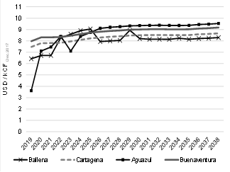
Source: Calculated by the authors based on[1]
Figure 2 Natural gas import and national well head projection prices
4.1.3. Transportation and its prices
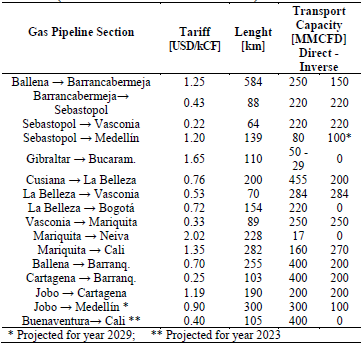
The transport trunk system consists of about 7,000 km, divided in this case into 110 sections of gas pipelines that connect the production fields or import ports with the consumption centers (see Fig. 3). The transport rates or tariffs are established at their maximum value by Comisión de Regulación de Energía y Gas (CREG) [Energy and Gas Regulatory Commission] [10,11] according to the physical characteristics of the gas pipelines (see Table 1).
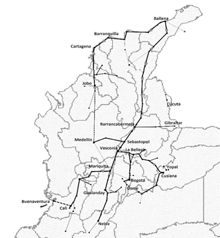
Source: Elaborated by the authors based on [1].
Figure 3 The natural gas transportation system in Colombia.
4.2. Results obtained from the simulation
With the monthly data projections for the January 2019 - December 2035 period, the set of matrices that would characterize the operation of the Colombian natural gas system was established (see section 3.3). The resolution of the model is achieved through the Simplex Method [12], using the GLPK command of the MathLab software. However, the optimization problem in linear programming can also be solved with any other relevant software available to the general public.
The solution consists of obtaining, for each period t, the vector x t that contains the production quantities in each of the source nodes (national production fields or import ports), the demand supplied (and not supplied) in each node, and the flows in each sections of the system (applying eq. 22). (Consider that it is possible to consult the most important variables of the real system in [13,14]). Some of the results achieved are found below:
4.2.1. Operating costs and rates
Fig. 4 shows the projection of the national operational cost of the natural gas service resulting from eq. (1). This projection shows a growing trend related to the increase in demand and prices, this one increasingly higher as more natural gas is imported.
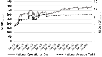
Source: The Authors.
Figure 4: National monthly operational cost projection and the national average rate for the natural gas service.
The national average rate obtained from eq. (6) shows a gradual increase in the next decade that is also related to the increase in natural gas prices, whether domestic or imported (see section 4.1.1). In the decade of the 2030s, this rate stabilized, as projected by international prices (see Fig. 2).
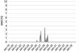
4.2.2. Shortage
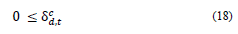
The model projects the magnitude of the unsupplied demand, which corresponds to the variable
 , accordingly with eq. (18). Between years 2026 and 2028 there would be rationing of up to 4 MMCFD (about 0.3% of the national demand, see Fig. 5), which is overcome by the year 2029 with the entry into operation of the Jobo-Medellín transport line (see Table 1). This deficit originates due to transport capacity limitations and not to supply limitations since the latter significantly exceeds the average demand (Fig. 1).
4.2.3. Transport flows
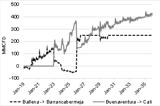
With the modeling exposed, and in particular with eq. (22), it is also possible to establish the flows in the different sections of the system to estimate potential expansion requirements of the transport capacity in the network sections. As an example, Fig. 6 shows the flow between the Atlantic Coast and an inland region of the country (Ballena → Barrancabermeja), and between the Pacific Coast and another inland region of Colombia (Buenaventura → Cali). In the first case, the bidirectional flow is evident as a result of the entry of new import sources in the years 2023 and 2026. In the second case, there is a progressive import through this port until the saturation of the transport capacity in the decade of the 2030s occurs, and its expansion towards the year 2035.
5. Conclusions
The work carried out considers a methodology to simulate a minimum cost, stable and long term operation of a natural gas system. The model used to simulate a natural gas transport network is comprised as a system of nodes that represent the supply sources and the consumption centers, interconnected through transport lines.
The mathematical formulation to characterize such an operation, which originally includes non-linear relationships between its variables, was transformed into a linear and matrix structure that allows its easy resolution, reducing computing execution times and allowing the use of common optimization software available to the general public. The methodology proposed in this work has the potential to be applied in other energy systems.
The approach applied in this study had the purpose of: i)- estimate the final costs and tariffs on the end user; ii)- establish the production of each source, the flows in the transport lines, as well as the demand supplied and not supplied in each of its nodes; iii)- using complementary algorithms, to determine the route followed by the gas through the system, as well as the effects of changes in the capacities of the elements of the system.
The results achieved in this work with the methodology detailed constitute reliable and relevant information for the analysis of energy systems (infrastructure construction needs, reliability in the provision of the service, user fees, optimization possibilities, among others), as well as for public policy makers to make investment decisions. From this work, new complementary models are being developed to assess the reliability of these energy systems, project competitive prices for national sources regarding import prices and others aiming at having new tools for planning natural gas and energy systems, in general.
Even in spite of the political difficulties that the energy interconnectivity with Venezuela is currently occurring, within the planning agenda of the next few years, the possibility of developing energy markets (electric and hydrocarbons) common among the Andean nations has been considered. Concerning this point, joint modeling of their networks would be necessary, as well as the verification of the convenience from an operational, reliability and economic points of view [15].

