


 English (pdf)
 Article in xml format
 Article references
 Send this article by e-mail
 Cited by SciELO
  Cited by Google
  Similars in
SciELO
Similars in
SciELO  Similars in Google
 Permalink
1. Introduction
Nowadays, there is a growth in the importance and attention that companies have given to the recovery of products or materials from customers, either to recover value or as after-sales services. This reverse process was already called Reverse Logistics [1] years ago. [2] affirm that RL is part of and becomes a fundamental part of the reverse supply chain, where the role played by manufacturers or producers is important, designing and implementing processes for the recycling and/or reuse of products or materials.
Different authors have conducted studies and research, to define what LI is, also called reverse distribution, retro logistics, or logistics of recovery and recycling. The most widely used is the one proposed by [3] in the Reverse Logistics Executive Council, defined as "The process of efficient and cost-effective planning, execution and control of the flow of raw materials, in-process inventory, finished goods and related information from the point of consumption to the point of origin to recover value or proper disposal". Nowadays, companies have been encouraged to design and implement Reverse Logistics (RL) systems [4]; according to [5], the main reasons why companies carry out RL are economic benefits, legal pressures, and the growing citizen culture regarding the issue of product return, reasons that coincide with what was stated by [6], who affirm that by practicing RL, enormous economic benefits are obtained for the company.
Consequently, researchers began to focus their efforts on designing RL systems, to attack the problems related to the mishandling and treatment of end-of-life products. One of the first applications of RL system design was related to the control and good management of hazardous materials. Thus, authors such as [7-10], carried out research to study specific reverse logistics networks for harmful waste such as hospital waste, lithium batteries, and dangerous household waste, developing Mixed Integer Linear Programming (MILP) models and including the stochastic component to determine the quantities to be transported and the optimal routes to be generated for the management of such waste.
Similarly, several authors have focused their efforts on designing reverse logistics networks for end-of-life products, such as [11,12], they researched to design reverse logistics networks for end-of-life products from the automotive industry, developing mathematical models of MILP and making use of various complementary algorithms, to determine the most efficient way for the collection and final disposal of waste from this industry. A potential opportunity has been identified in the application of reverse logistics theories by applying them to the collection and disposal of pesticide residues. Authors such as [13-15], have conducted studies in which they agree that there has been an increase in concern about the consequences and risks that empty pesticide containers and packaging can present in terms of both health and the environment.
Consequently, authors such as [16-18] investigated the attitude and behavior of farmers on the use and waste of pesticides in western Iran, where the results show that farmers had not been trained on the use and disposal of pesticides.
Given these considerations, this article shows the results of a research developed in the irrigation district of USOCHICAMOCHA - Boyacá, Colombia, where there is currently a problem of inadequate handling and treatment of pesticide wastes by farmers, in addition to not having a defined reverse logistics process. Consequently, the objective of the research is to propose and evaluate different models for the correct planning and execution of the collection days of empty pesticide containers and packaging, for which a study was developed that applied two quantitative tools Mixed Integer Linear Programming and Discrete Event Simulation, in order to observe which of them best models the process under study and also offers the best alternatives to implement possible improvement scenarios.
In this sense, this article is structured as follows: section two (2) shows the literature review that was conducted on the subject of reverse logistics, then section three (3) shows the methodological structure, where each of the phases followed for the development of the research is explained. Then, in section four (4) the main results of the research are shown in a synthesized way, as well as the result of the application of each one of the modeling tools. Finally, section five (5) presents the main conclusions, product of the research developed.
2. Literature review
A literature review conducted by [19], initially identifies the most relevant topics or with greater attention among the authors of publications in the field of reverse logistics, where it is observed that the most important topics are green logistics, sustainability, product life cycle, product return, remanufacturing and reverse logistics network design. [20] found the quantitative techniques adding others with high use such as Mixed Integer Nonlinear Programming (MINLP), Mixed Integer Fuzzy Programming, Markov Chains, and Full Fuzzy Programming.
Complementary to this, an analysis of the quantitative techniques used by various researchers in recent years was carried out, making an exhaustive search of articles whose objective was to design RL networks for different types of waste, making use of mathematical tools. Table 1 shows that there is a tendency to use MILP as the main tool for the design of the networks since this tool offers researchers the opportunity to find optimal solutions to the models. Likewise, there is an important use of Goal Programming (GP) to establish the RL models, offering an additional alternative in the fulfillment of different objectives within the same model. Some research that use Stochastic Programming (SP) for the modeling of random variables are highlighted, including the combination of mathematical techniques for the total development of the model.
Table 1 Mathematical tools in RL research.
| Authors | MILP | MINLP | PM | AEC | SP | AG | GP | FP | VRP |
|---|---|---|---|---|---|---|---|---|---|
| [21] | X | ||||||||
| [22] | X | ||||||||
| [23] | X | X | |||||||
| [11] | X | ||||||||
| [4] | X | X | |||||||
| [10] | X | X | |||||||
| [24] | X | ||||||||
| [25] | X | X | |||||||
| [26] | X | ||||||||
| [27] | X | ||||||||
| [28] | X | X | |||||||
| [9] | X | ||||||||
| [8] | X | ||||||||
| [29] | X | ||||||||
| [22] | X | X | |||||||
| [30] | X | ||||||||
| [31] | X | ||||||||
| [32] | X | X | |||||||
| [33] | X |
Source: authors
3. Methodology
The research developed is a case study following the guidelines set out by [34], where it has two levels of research scopes: descriptive and experimental. The methodological phases followed for the development of the research were stipulated according to each of the quantitative tools used as follows:
3.1. Phase 1. Deterministic mathematical model
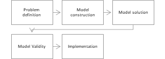
In this phase, a Mixed Integer Linear Programming (MILP) model was developed, following the guidelines of [35] described in Fig. 1:
Initially, through direct observation, a description of the reverse logistics process that is currently carried out for empty pesticide containers and packaging in the irrigation district is made, identifying all the variables and parameters that interfere with the process, in order to determine the objective to be placed in the mathematical model.
Subsequently, the MILP model is built, including continuous variables such as quantities collected in Kg and decision variables such as the possibility of opening new collection centers. Initially a codification of the identified variables and parameters is performed. The objective function equation and the constraint equations that complement the mathematical model are determined.
Once the mathematical model is built, the solution is developed, starting with the collection of the necessary information through field visits and accompaniment to the collection days and data provided by the companies in charge of collecting pesticide containers and packaging. Then, the model was solved through the specialized software for operations research LINGO®. Finally, based on the solution, a validation of the model is performed, verifying initially that the results obtained are consistent with the reality of the process under study and also evaluating possible scenarios for improvement of the system.
3.2. Phase 2. Simulation model
Subsequently, a discrete event simulation model was developed following the methodology of [36] described in Fig. 2.
The description of the reverse logistics process carried out in the previous phase serves as the basis for the creation of the simulation model, where it is initially evaluated whether the variables and characteristics included in this characterization are relevant for the development of the simulation model.
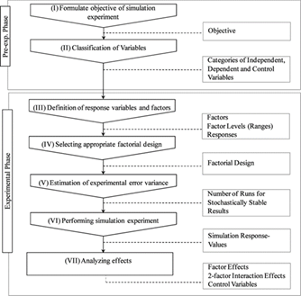
This model starts by mapping the area under study and identifying the collection routes of empty pesticide containers and packaging used by the company.
Next, the construction of the simulation model begins, starting with the preliminary construction of the layout under the specialized software FlexSim®, according to the description of the process obtained in the previous stage. Subsequently, according to the stipulations of [37], a time study was carried out for each of the activities that are part of the reverse logistics process under a continuous timing criterion, managing to collect 93 data for each of the activities. Once the data were collected, they were inserted in the Stat: Fit tool of the specialized software Promodel®, where the best probability distribution representing each of the activities was determined, verifying it through goodness-of-fit tests such as Kolmogorov-Smirnov and Anderson Darling.
Afterwards, with the probability distributions defined, these were implemented in the preliminary model and the final adjustment was made to the model in visual terms, performing the stabilization of the model as described by [38].
Finally, the verification and validation of the final model were performed, choosing as variables for this process the total time of the reverse logistics process, in which a pre-sample of 10 runs of the model was performed in order to determine the number of replicates necessary for the validation, where finally the sample gave 15 replicates, performing an analysis of means through a t Student test for independent samples, corroborating if there is equality in the means of the real system and the model developed in FlexSim.
Finally, experimentation with the model is carried out, defining possible improvement scenarios, establishing a confidence level of 95% and a significance level of 5% for each of the scenarios.
4. Results
4.1. MILP Model
4.1.1. Set and indexes
I: Set of farm or property with index
J: Set of Final Disposal Alternative type with index j
K: Set of waste type (Packing or packaging) with index k
L: Set of periods in which the capacity with index l varies.
M: Set of collection and disposal period with index
4.1.2. Parameters
CTX m = Cost per kilogram of pesticide residue transported and kilometer traveled in the period m
CTY jm = Cost per kilogram of pesticide residue transported and kilometer traveled from the collection center to disposal alternative j in the period m
DTX i = Distance in kilometers from the farm i to collection center
DTY j = Distance in kilometers from the collection center to the final disposal alternative j
CG ikm = Kilograms of waste k generated by farm i in period m
CDISP jk = Processing capacity of waste k in disposal alternative j (kg)
CVREC m = Capacity in kilograms of the collecting vehicle in period m (kg)
CVDISP m = Vehicle capacity for transport to final disposal in period m (kg)
CICA= Initial capacity of the collection center (kg)
4.1.3. Variables
X ikm = Quantity of waste type k to be collected and sent from each farm type i to the collection center in period type m (kg).
Y jkm = Quantity of waste type k to be sent from the collection center for final disposal alternative type j in period type m (kg)
CAPCA m = Storage capacity of the storage center in the period type m (kg)
Objective function and constraints
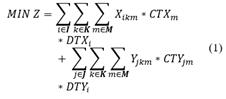
Subject to:


Eq. (1) indicates the objective function of the problem that minimizes the total cost of the process of collection and final disposal of pesticide containers and packaging, which contains both the cost of transportation and the cost of the operators involved in the process, as well as the distances from each of the farms to the collection center and the distance between the collection center and each of the places where the different alternatives for final disposal are carried out.
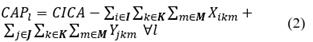
Restriction (2) calculates the capacity of the collection center in each collection period, which depends on the quantities collected and taken to the final disposal. Eq. (3) ensures that the total quantities collected in a period do not exceed the available capacity of the collection center, to guarantee that no pesticide containers and packaging are left lying around or out of control. In addition to this, Eq. (4) guarantees that the quantities collected in each farm and each period are those identified as generated and ensures that there are no uncollected residues in the farms.
Eq. (5) guarantees that the total amount of pesticide residues collected at the farms and taken to the collection center in each period is the same amount of residues that will be transported to each of the disposal alternatives in the same period, guaranteeing that no pesticide residues are in storage or unprocessed at the collection center. Constraint (6) takes into account the capacity of each of the disposal alternatives in order not to send more waste than they can receive for processing. Eqs. (7) and (8) take into account the capacity of vehicles to collect waste on the farm and to take it to each disposal alternative, respectively. Eqs. (9-11) are non-negativity restrictions that guarantee that the quantities to be collected, transported to final disposal, and stored in the collection center are positive.
4.2. Discrete event simulation model
Initially, for the simulation model, a description of the activities that make up the process of collection and final disposal of empty pesticide containers and packaging was carried out, in addition to a time study. Fig. 3 shows the diagram of the reverse logistics process currently being carried out in the area under study, as well as the standard times for each of the activities, in which it can be seen that the longest time is spent on transportation to each of the farms, since the distances between farms are long and the geographic and road conditions are not optimal.

Table 1 Probability distributions stochastic activities
| Variable | Probability distribution | K-S | Anderson Darling | % adjustment | ||
|---|---|---|---|---|---|---|
| ST | CV | ST | CV | |||
| Displacement to each generating farm | Exponential | 0,05 | 0,13 | 0,49 | 2,49 | 79,2 |
| Transportation to the collection point on the farm | Reverse Weibull | 0,06 | 0,13 | 0,6 | 2,49 | 100 |
| Waste pre-inspection | Reverse Weibull | 0,06 | 0,19 | 0,25 | 2,49 | 99 |
| Transport of waste to the vehicle | Reverse Gaussian | 0,05 | 0,13 | 0,36 | 2,49 | 100 |
Source: Authors. ST=Statistical, CT=Critical Value
The discrete event simulation model was implemented taking into account the randomness of each of the identified variables. Table 1 shows the adjustment of probability distributions to each of the variables, which were verified through goodness-of-fit tests, the results of which are also shown.
Once the simulation model was obtained, it was validated through a test t for two samples assuming equal variances. The validation variable chosen was the total time of the process of collecting empty pesticide containers and packaging. A confidence level of 95% and an admissible error of 5% was established for the FlexSim model, and with this criterion, 10 initial runs were carried out to determine the minimum number of runs necessary, which was 15:

Table 2 Test t for validation
| Flexsim | Real | |
|---|---|---|
| Mean | 369,99 | 364,8 |
| Variance | 310,27 | 1268,59 |
| Observations | 15 | 3 |
| Hypothetical difference of means | 0 | |
| Degrees of freedom | 2 | |
| Statistical t | 0,246 | |
| P(T<=t) a queue | 0,414 | |
| Critical value t (a queue) | 2,919 | |
| P(T<=t) two queue | 0,828 | |
| Critical value t (two queue) | 4,302 |
Source: Authors
Table 3 Test t for validation
| Current | Scene 1 | Scene 2 | |||
|---|---|---|---|---|---|
| Operator | Operator 1 | Operator 2 | Operator 1 | Operator 2 | |
| Wait | 80,79% | 77% | 79,57% | 82,85% | 77,59% |
| Transportation to the collection point on the farm | 6,42% | 6,02% | 5,58% | 6,27% | 5,37% |
| Transportation to the vehicle | 7,03% | 2,72% | 1,08% | 2,77% | 2,72% |
| Sort | 1,54% | 1,18% | 1,18% | 2,03% | 1,89% |
| Pre-inspection | 4,23% | 12,64% | 12,64% | 6,08% | 12,43% |
| Vehicle | Vehicle | Vehicle 1 | Vehicle 2 | ||
| Farm to farm transportation | 73,70% | 81,50% | 74,72% | 85,92% | |
| Waste recolection | 19,50% | 8,02% | 18,47% | 3,35% | |
| Idle | 6,80% | 10,42% | 6,73% | 10,61% | |
| Overall process time (min) | 368,64 | 314,54 | 199,78 | ||
| Decrease of time (min) | 0 | 54,1 | 168,86 | ||
| Percentage improvement | 0% | 15% | 46% | ||
Source: Authors
Where n is the total number of replicates to be carried out, s is the standard deviation of the pre-sample, t is the theoretical value of the student t distribution with n-1 degrees of freedom, and a probability α and e refers to the admissible error. Table 2 shows the results of the test t developed for the validation, where it can be observed that the critical zone of this test is between -4.3 and +4.33, and as the statistic t is within this interval, it is concluded that there is no significant difference between the total time of the collection process of the two systems, not rejecting the null hypothesis of equality of means, so it is established that as there is no difference, the model developed in FlexSim is validated concerning the real system.
Finally, experimentation is carried out with the discrete event simulation model, proposing two scenarios for improving the system. The first scenario is characterized by the addition of an operator to support the pre-inspection and collection activities of the waste generated in each farm. The second scenario is characterized by the addition of a collection vehicle that, together with the second operator added in scenario 1, will take an alternate route to cover 6 of the 11 farms that generate waste in the irrigation unit. Table 3 shows the results for the data output analysis of the different scenarios.
The most representative improvement can be observed in the decrease of the processing time in each scenario, being number 2 the most favorable with 168.86 min, concerning the current system model, this scenario represents an improvement in the process of 46%. The proposed model produces the best and most viable conditions adaptable to the real system that generates the greatest reduction in the total time of the process of collection and collection of pesticide residues.
5. Discussion
The MILP mathematical model developed yields the minimum quantities of empty pesticide containers and packaging to be collected in each of the farms for each collection period, where it is evident that for all periods in each farm, the model generates the same result only differentiating by type of waste, achieving in total the collection of a greater quantity of containers than packaging, with a total of 1,292.3 kg of containers and 1,106.6 kg of packaging. Likewise, the results show the quantities to be taken to each of the final disposal alternatives, where only the eco-processing option is chosen for packaging and recycling containers in the same quantities for all periods.
The proposed model increases by 36% the number of empty pesticide containers and packaging to be collected, compared to the average amount currently being collected on all farms in the district (1760 kg of waste). Finally, this model proposes several improvement scenarios where it is evident that the capacity of the collection center, collection vehicle capacity, and disposal vehicle capacity, currently at 12,000, 3,000, and 8,000 kilograms respectively, could be reduced to 2,399 kilograms or more since the quantities being generated on the farms in the district are lower than this proposal, to reduce costs and have greater control over the quantities being stored.
In comparison with the results obtained through the discrete event simulation model, it is evident that the model represents in a better way the real operation of the inverse logistics process, however obtaining results with totally different approaches to the MILP model since the simulation model does not determine the quantities to be collected, but on the contrary, it does represent the stochastic variables and includes the variability of the process, which the deterministic model does not. On the other hand, it is evident that the scenarios proposed in the simulation model are focused on the implementation of resources to reduce the total time of the process, which does not guarantee that a greater amount of pesticide residues will be collected, but the MILP model does, whose objective and improvement proposals are focused on increasing the quantities to be collected.
6. Conclusions
The results obtained show that the two models developed present both advantages and disadvantages and do not fully represent the real operation of the reverse logistics process of empty pesticide containers and packaging since, despite being very powerful quantitative tools, they focus on particular objectives, ignoring some of the characteristics of the real model.
Likewise, it can be observed that the process under study needs both a deterministic and a stochastic representation to achieve accurate results and to be able to propose significant and efficient improvements to the process. Initially, it is considered important to include variables referring to quantities to be collected and taken to final disposal, as well as the evaluation through binary variables of the opening of new collection centers, which is achieved through deterministic models, but it is also necessary to include the variability or randomness of variables in order to represent the process to a greater extent and for the results obtained to have greater reliability, which is achieved through stochastic models.
Finally, it can be inferred that a possible option to represent the reverse logistics process of empty pesticide containers and packaging is to develop a model that includes two phases, on the one hand, the deterministic one to achieve optimal results combined with a model that includes stochastic variables.

