


 English (pdf)
 Article in xml format
 Article references
 Send this article by e-mail
 Cited by SciELO
  Cited by Google
  Similars in
SciELO
Similars in
SciELO  Similars in Google
 Permalink
Introduction
Tilapia is the second most important fish in aquaculture after carp. Global production of Oreochromis niloticus reached 3,670,260 tons in 2014 (FAO, 2016). Furthermore, Oreochromis spp. are the most economically important aquaculture species in Colombia (Ministry of Agriculture and Rural Development of Colombia, unpublished data), and this country was the second largest exporter of fresh tilapia fillet to the United States in 2015, with 5,329 tons valued in USD $44,119,211 (NMFS, 2016).
Colombia has a long history of successive introductions of tilapia. Importation of O. niloticus began around 1979 to promote aquaculture, followed by red varieties of Oreochromis mossambicus and Oreochromis urolepis, Nile strains, and red hybrids (Gutiérrez et al., 2012). As a result, several tilapia species are cultured in this country. However, maintaining genetic variation is important because of its critical role in a population’s adaptative potential to cope with variable environmental conditions, and its usefulness when genetic improvement through selective breeding is anticipated (Lind et al., 2012).
Aquaculture stocks derived from small founder populations, show after few generations, loss of genetic diversity as well as depression related to inbreeding (Doyle, 2016). Therefore, the gene pool needs to be refreshed periodically (McKinna et al., 2010). For tilapia, total female fertility and male reproductive success are affected by the level of endogamy (Fessehaye et al., 2009). Thus, it is important to monitor broodstock genetic diversity in aquaculture farms responsible for fry production (Petersen et al., 2012). Microsatellites are among the best genetic markers for analyzing pedigree, population structure, genomic variation, and evolutionary processes, as well as for verifying the quality of selective breeding programs in aquaculture (Abdul-Muneer, 2014).
Genetic diversity of Oreochromis spp. has been extensively studied using microsatellites worldwide (Petersen et al., 2012; Gu et al., 2014). Diversity metrics such as heterozygosity, allelic richness and inbreeding coefficient are highly variable between studies. Previous work by Brinez et al., (2011) evaluated the genetic diversity of six populations of red hybrid tilapia from several regions of Colombia. However, the genetic diversity and structure of broodstocks from the Antioquia region remains unstudied.
Accordingly, the purpose of this study was to assess the genetic variability and population structure of broodstocks in the most important tilapia hatcheries in Antioquia, Colombia. In addition, we discuss current trends and directions for future research in the study of genetic diversity of tilapia using microsatellites.
Ethical considerations
Handling procedures followed the section seven of the Aquatic Animal Health Code about welfare of farmed fish (OIE, 2016).
Tissue sampling
The farms were selected according to the following criteria: a. they had their own breeders and hatcheries, and b. their high contribution to tilapia production in Antioquia (Colombia). Terminal tailfin fragments were collected randomly from tilapia broodstock in one Nile and three red tilapia farms. Samples were stored in 98% ethanol until processing.
DNA isolation and amplification
Genomic DNA was extracted from samples using DNEasy® blood and tissue kits in the QIAcube® automated system (QIAGEN), in accordance with manufacturers’ protocols. Total DNA was quantified, and its purity (260-nm/230- nm ratio) was determined using a NanoDrop® spectrophotometer (Thermo Fisher Scientific). Next, DNA integrity was visualized with 1.2% agarose gel using SYBR® Safe gel stain (Thermo Fisher Scientific).
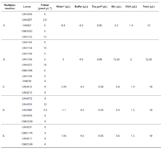
Twenty-four microsatellite loci located in 13 different linkage groups were analyzed with forward primers tagged with fluorochrome markers FAM, VIC, NED, or PET (Table 1). Five sets of primer tags in multiple reactions (Table 2) were amplified, such that all fragments could be uniquely marked and separated within a single capillary without overlap. PCR was carried out in reaction volumes of 10.0 to 12.3 µl with a thermal profile of initial denaturing at 94 °C for 15 min, followed by 30 cycles of 30 s at 94 °C, 90 s at 56 °C, 90 s at 72 °C, and 10 min at 72 °C. Fragment lengths were determined with a GeneScan® 500 ROX® Size Standard (Applied Biosystems) in an Applied Biosystems 3130 automated capillary genetic sequencer. DNA sizing and quality allele calls were analyzed with GeneMapper software version 4.0 (Applied Biosystems).

Data analysis
Data were transformed and alleles were grouped using TANDEM software version 2.0 (Matschiner and Salzburger, 2009). SPAGeDi software version 1.5 (Hardy and Vekemans, 2002) was used to calculate the number of alleles, effective number of alleles, observed heterozygosity, expected unbiased heterozygosity (Nei, 1978), allelic richness, and individual endogamy coefficient. Genepop software version 4.1 (Rousset, 2008) was used to determine deviations from Hardy- Weinberg equilibrium (HWE) across populations within loci and across loci within populations via the Markov chain method, with heterozygote deficit being specified as the alternative hypothesis. Markov chain length was 1,000 iterations plus 100 subsequent groups of 2,000 iterations. Genepop version 4.1 (Rousset, 2008) was used to analyze allele fixation and linkage disequilibrium via the G-test with 10,000 dememorizations, 100 groups, and 5,000 iterations per group. Genetix software version 4.02 (Belkhir et al., 1996) was used to calculate the number of private alleles per locus, Wright’s fixation index (FST) (Weir and Cockerham, 1984), and Nei’s distance (Nei, 1972). To detect artifacts (“stuttering”), loss of alleles, and null alleles, Micro-Checker software version 2.2.3 was used (Van Oosterhout et al., 2004). Hierarchical subdivision of genetic diversity was determined via Analysis of Molecular Variance (AMOVA) using Arlequin software version 3.5.2.2 (Excoffier and Lischer, 2010). To determine the number of groups and to assign individuals to specific groups, Structure software version 2.3.4 was used (Pritchard et al., 2000). The analysis was performed in accordance with recommendations of Gilbert et al. (2012). For Markov chain Monte Carlo, 100,000 burn-in iterations and repetitions for each run, were used. To confirm parameter suitability, value convergence in the statistical summary was determined, as recommended in the Structure User Manual (Pritchard et al., 2010). Twenty independent replicas with one to seven groups were run in the Structure software program. To select the number of clusters (K), the method of Evanno et al., (2005) was applied by using the online software application Structure Harvester version 0.6.94 (Earl and vonHoldt, 2012).
Results
Between 32 and 47 fish per farm were genotyped. Two microsatellites (UNH208 and UNH222) could not be amplified. The remaining 22 microsatellites were polymorphic. Across the four broodstocks, the number of alleles per locus varied from four (locus OMO032 in all four broodstocks) to 12 (UNH118 in red 1 broodstock). Average number of alleles per locus was between 5.77 (Nile) and 7.91 (red 3). The highest total number of alleles was 17 in locus UNH211, and the lowest was 4 in locus OMO032. Allelic range was 101 to 143 (locus UNH207), and 303 to 359 (locus OMO175). Allelic range amplitude varied from six (locus GM234) to 88 (locus GM407). Average effective number of alleles was always lower than observed number of alleles and fell between 3.37 (red 3) and 4.03 (Nile). Half of the loci (44/88) showed significant deviations from HWE, and 42 of these loci showed heterozygote deficiency. Loci OMO032, OMO194, and UNH159 were in HWE in all four broodstocks. Loci OMO228, UNH106, UNH160, and UNH216 were in HWE in three of the four broodstocks.
At least one private allele per broodstock was found in the 20 loci (except in GM234 and OMO032), and locus OMO228 had seven private alleles. The Nile population had the highest number of private alleles (22). Micro-Checker analysis showed evidence of null alleles in loci GM407, OMO175, UNH104, UNH108, UNH118, UNH123, UNH124, UNH129, and UNH166.
Eliminating loci with null alleles, linkage disequilibrium analysis for all populations showed six loci pairs with p<0.05. Loci pairs UNH159-OMO194 and UNH207-UNH231 had infinite x2 values and highly significant p values. Thus, loci UNH159, OMO194, and UNH207 were excluded from further analysis. Table 3 shows the genetic diversity descriptors per broodstock for the 10 microsatellites, excluding loci with null alleles and linkage disequilibrium (GM234, OMO032, OMO039, OMO228, UNH106, UNH160, UNH172, UNH211, UNH216, and UNH231). The calculated value of unbiased expected heterozygosity varied depending on the microsatellite marker group (Table 4). Differences between calculations were generally smaller when 10 and 13 microsatellite markers were used than when 22 markers were used. Expected heterozygosity based on Hardy-Weinberg proportions ranged between 0.6504 (Nile) and 0.686 (red 2). Observed heterozygosity was different from the expected heterozygosity in all four broodstocks (p=0.000, standard deviation =0.000).
Table 3 Genetic diversity per broodstock from 10 microsatellites, excluding null alleles and loci with linkage disequilibrium.

Na - number of alleles; Nae - effective number of alleles; AR - allelic richness; Fis - individual endogamy coefficient.
Table 4 Expected heterozygosity (He) and observed heterozygosity (Ho) per population calculated from different microsatellite groups.

The FST value for all broodstocks together (excluding null alleles and linkage disequilibrium) was 0.0777 (95% confidence interval, 0.05763 to 0.09718), reflecting the low average substructuring. AMOVA results showed that the greatest variation was between individuals. Variation percentage from the source “between groups” was very low (0.80%). Sources “between broodstocks within groups” and “between individuals within broodstocks” showed negative variation percentages, because their values could be close to zero (Table 5).
The trend of the logarithm curve for the probability of number of clusters K began to plateau at K = 3, with a value of -4049.155. However, the most appropriate number of clusters based on estimates of ΔK was two (ΔK = 798.053). Figure 1 shows a graphical representation of the assignment of each individual to K = 2, 3 or 4. Nile broodstock was the only that retained an assignment proportion greater than 90% in just one cluster among all values of K evaluated (results for K = 5, 6, and 7 not shown). In red broodstocks, the maximum assignment proportion decreased with an increase in K value. Finally, red broodstocks were closer to each other (Nei’s distance: 0.03 to 0.08), than they were to the Nile broodstock (Nei’s distance: 0.433 to 0.54).

Discussion

Figure 1 Assignment of each individual from the four broodstocks to K = 2, 3, or 4. Each color represents one cluster. Length of each bar was the estimated assignment proportion of a particular cluster. Graphs were obtained from the Structure software package.
On a global level, different panels of microsatellites have been used for diversity analysis of wild and farmed populations of Oreochromis sp. (particularly of O. niloticus, see Table 6). However, these results are not comparable across studies. First, the estimation of levels of population genetic diversity (allelic richness, expected heterozygosity, coefficient of inbreeding), structure (FST), and genetic distances (Nei) from microsatellite data is depending on number of loci and the strategy of marker selection (Orozco-terWengel et al., 2011; Blanco et al., 2012; Queirós et al., 2015). Second, there are differences in detection and scoring of microsatellites between techniques such as: agarose gel, slab gel and capillary electrophoresis (Vemireddy et al., 2007; Stewart et al., 2011). Third, most studies did not test the neutrality of markers, the occurrence of null alleles and linkage disequilibrium. Fourth, the comparisons among populations with appreciable size differences between alleles may be biased because longer microsatellite alleles mutate at a higher rate (Putman and Carbone, 2014). Finally, although some of the microsatellite loci used in the present study were also used in previous works, this is the first report using this panel. Our contrasts therefore need to be interpreted with caution.
A median of nine microsatellites have been used in genetic diversity studies for Nile and red tilapia populations (range: 4-20 markers, see table 6), which represents a slightly smaller number than the one of microsatellites used in the present study (10). According to Koskinen et al. (2004), a possible disadvantage of using a small number of loci is an increased standard deviation of genetic distances across populations.
The studies listed in Table 6 found that the mean number of alleles per locus per population ranged from three (Karuppannan et al., 2013) to 50 (Bhassu et al., 2004) with a median of 5.87, which is in accordance with the present results. However, we obtained decreased values of the mean number of alleles compared to previous studies in Colombia and Brazil (6.45 in the present study vs. 8.37 in Brinez et al., 2011 and 10,46 in Petersen et al., 2012, respectively). Nineteen different panels of microsatellite loci in several tilapia populations worldwide showed expected heterozygosity values between 0.170 Bezault et al. (2011) and 0.968 Bhassu et al. (2004), and observed heterozygosity values between 0.150 (Dias et al., 2016) and 0.90 (Hassanien and Gilbey, 2005) with a median of 0.686 and 0.649, respectively (Table 6). Our results of He (0.6504 to 0.686) and Ho (0.601 to 0.649) are consistent with these reports.
The farms sampled in the present study did not keep records of broodstocks origin and pedigree, and the genetic background of broodstocks was unknown. Moreover, the farmers carry out replacement of broodstocks based on mass selection for coloration and growth (red or Nile tilapia, respectively) of some groups that are not sex-reversed derived mostly from their own farms. These practices could decrease the genetic diversity of broodstock after only a few generations. For example, Romana-Eguia et al. (2005) reported a reduction in the mean number of alleles (from 10 to 7.4) and mean He (from 0.752 to 0.691) in selected and control stocks of mass-selected Nile tilapia after four generations.
Comparisons of the deviations from HWE obtained in the present work with those of previous studies (Table 6) confirms that some wild populations and unselected stocks of tilapia conformed to the HWE (Romana-Eguia et al., 2004; Bezault et al., 2011; Sukmanomon et al., 2012), while departure from HWE equilibrium was detected in most of the farmed populations due to a significant deficit of heterozygotes. Deviation of the HWE in hatchery populations could be attributed to the aquaculture practices because a limited number of adults are spawned and an unequal sex ratio is applied (Napora- Rutkowski et al., 2017). The FIS values obtained in this study (0.031-0.121) indicate a deficit of observed heterozygotes. These results reflect those obtained previously by Rutten et al. (2004), Nyingi et al. (2009), some populations in Bezault et al. (2011) and Gu et al. (2014). In contrast, Melo et al. (2006), Moreira et al. (2007) and Dias et al. (2016) found negative values of FIS (see Table 6). Furthermore, our results are similar to the positive values of FIS in tilapia populations from Colombia (FIS =0.345 in Brinez et al., 2011) and Brazil (FIS = 0.160-0.330 in Petersen et al., 2012; FIS = 0.192-0.401 in Rodriguez-Rodriguez et al., 2013).
The FST value of 0.078 (95% confidence interval, 0.05763 to 0.09718) obtained in this study suggests a low level of genetic differentiation. This result is comparable with the FST values of tilapia populations from Philippines (FST = 0.069, Romana-Eguia et al., 2004), Egypt (FST = 0.035, Hassanien and Gilbey, 2005), Africa (FST =0.09, Bezault et al., 2011), Thailand (FST = 0.087, Sukmanomon et al., 2012) and India (FST = 0.089, Shyamala et al., 2014). On the contrary, six commercial stocks of tilapia from Brazil exhibited large genetic difference (FST = 0.326, Melo et al., 2006).
The AMOVA results in the present study indicated that almost the entire variation occurred between individuals. These findings differ from those obtained by Brinez et al. (2011) for four Colombia provinces; excluding Antioquia, because they reported variation percentages of 17.32% between populations, 28.55% within populations, and 54.12% between individuals. The AMOVA results of the present study were similar to those of Romana-Eguia et al. (2004), who reported 99.33% variation between individuals and only 0.00331% between groups of red and Nile tilapia. In contrast, Bezault et al. (2011) found in natural populations of O. niloticus that 49.8% of the genetic variability was partitioned among hydrographic basins and 3.5% was detected among populations within basins.
We found evidence of null alleles at nine of 22 loci. This situation represents the absence of a PCR product due to a mutation in the region flanking the microsatellite. Also, it creates a false homozygosity reading in individuals that could be heterozygotes and, therefore, introduces biases in estimates of genetic diversity and differentiation across populations (Chapuis and Estoup, 2007). The presence of null alleles in microsatellite data of tilapia have been previously reported by Nyingi et al. (2009), McKinna et al. (2010), and Sukmanomon et al. (2012). Our result showed that after eliminating loci with null alleles the He values decreased. However, Bezault et al. (2011) identified in natural populations of tilapia that the exclusion of loci with potential null alleles had minor effects on FIS.
Linkage disequilibrium is the non-random association of alleles at distinct loci. It creates pseudo- replication for analyses in which loci are assumed to be independent samples of the genome. In order to avoid increased Type I error, one locus in the pair should be discarded if significant disequilibrium is found consistently between loci (Selkoe and Toonen, 2006). Therefore, we discarded the loci UNH159, OMO194, and UNH207. Nevertheless, after eliminating these loci the He values slightly decreased. Sukmanomon et al. (2012) and Rodriguez-Rodriguez et al. (2013) observed linkage disequilibrium in different pairs of microsatellite loci in tilapia. However, these authors did not apply any correction to the data. Conversely, McKinna et al. (2010) found no evidence to suggest that four microsatellite loci used in their tilapia study deviated from linkage equilibrium.
In the present study, the most appropriate number ΔK value was obtained for K= 2 (i.e., one red and one Nile cluster), and the values of Nei’s distances were higher between the three red and the Nile broodstocks. This outcome is contrary to that of Shyamala et al. (2014), who found a Nile tilapia population clustered with red tilapias due to breeding management schemes. Nonetheless, our results are similar to those of Romana-Eguia et al. (2004), in which Nile tilapias formed a distinct cluster from red tilapias.
In conclusion, ten microsatellite loci allowed the characterization of the genetic diversity and structure of three red and one Nile tilapia broodstocks from Antioquia, Colombia. This molecular analysis suggests that the four broodstocks are not affected by major loss of genetic diversity and it shows a clear separation between three red and the Nile broodstocks. Our results provide basic information that could be helpful for the management of tilapia hatcheries and the design of future breeding schemes. We would encourage researchers to standardize and calibrate a panel of microsatellite loci (including adaptive and neutral markers) in multiplex PCRs for tilapia that helps the comparison of information.
Table 6 Comparison of results obtained by previous microsatellite studies in wild and cultivated tilapia populations. No. of popul - number of population; Ho - observed heterozygosity, He - unbiased expected heterozygosity; FIS inbreeding coefficient; FST - Wright’s fixation index, gen - generations, CI - confidence interval.


