


 English (pdf)
 Article in xml format
 Article references
 Send this article by e-mail
 Cited by SciELO
  Cited by Google
  Similars in
SciELO
Similars in
SciELO  Similars in Google
 Permalink
I. INTRODUCTION
Today, Information and Communication Technologies (ICT) provide multiple tools for learning mathematics that are necessary for learning complex numbers. Complex numbers have applications in different fields, such as engineering (description of electrical circuits and electromagnetic waves), physics, chemistry, biology, mathematics and statistics, among others. Several concepts that include complex numbers require visual comprehension that is difficult to understand in a guide book or in a lecture. Using interactive tools for understanding this topic allows the student to comprehend the topics better.
All new technologies allow an increasingly important development in each of the daily activities, use them as an important tool to acquire or develop knowledge makes the application of theoretical concepts are simpler, and ICTs become an entertaining way to learn. It is essential that in order to obtain greater interaction with the new environments for the learning of complex numbers, we have previous knowledge on the subject and on the use of the tools to be used, in this case MATLAB and GeoGebra.
MATLAB is a mathematical software tool that uses its own programming language; it was created in 1984 in Albuquerque, Nuevo México, by a mathematician and programmer named Cleve Moler, and its name comes from the abbreviation of the words MATrix and LABoratory. The latest stable version is the R2018a, released in March of 2018. GeoGebra is a mathematical software application specialized in geometry, algebra and calculus. It is a free software, which makes it accessible to more people, and presents a friendly graphic environment simpler for the user. It was created in 2002 by Markus Hohenwarter from the University of Salzburgo, Austria, as his master's thesis, and its name comes from "Geo" from Geometry and "Gebra" from the Fundamental Theorem of Algebra. The most recent version is 6.0.465.0, launched on May of 2018.

Like this representation, it is possible to graph the results by means of the following form [8]:
II. METHODOLOGY
The methodology used during the development of the research is presented below. The potential of interactive systems in mathematics education and the tools proposed for a better understanding of complex numbers are discussed.
Learning complex numbers can often be a complex task for students and the general public [1], [2]. However, technology allows developing learning in an interactive way [3]. The irruption of information and communication technologies (ICT) "as an educational tool represents a turning point in the way in which learning [...], breaking with rigid schemes and traditional teaching has been done, to adopt other ways of building, managing and transmitting knowledge" [4].
Technological tools like MATLAB, GeoGebra [5], SciLab, Wolfram Alpha, and others evolve every day to provide better content, power and efficiency at the time of plotting or manipulating mathematical content [6]. Among the many tools that can be used, we have chosen MATLAB and GeoGebra, which will show the process of developing basic and some complementary operations with complex numbers, each one with its advantages and differences, to provide the user with information to choose the preferred tool.
III. RESULTS
Below are the results obtained after the application of some examples using the proposed tools: MATLAB and GeoGebra.
A. Complex numbers in MATLAB
The environment of MATLAB is designed to be used directly through commands. In addition, it is possible to graphically display the results [7]. We can create a complex number in MATLAB in the following ways [1]:
>>plot(z1,’og’,’MarkerSize’,7,’ Marker Face Color’,’g’); text(real(z1)+0.08,imag(z1), ‘12 + 7i’)
>> grid on
>> title (' Representation of an Imaginary number)
MarkerSize - Specifies the marker pixel size
text: Allows you to assign a text to the point that was plotted, in this case, drawing the coordinates of the number plotted to establish its correct position.
grid on: Draws a grid on the graph to distinguish the position of the graphed points more easily.
title: Allows you to assign a title to the graph.
figure: Receives as a parameter a number that will assign an order to the drawn figures.
hold on: Allows drawing some of the points in a fixed way, without the possibility of being drawn when drawing another new point or updating the graph.
Operations between complexes: As an example, below, we will show operations established for complex numbers, such as basic operations and module, conjugate, complex number roots, and polar form [9].
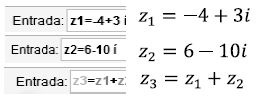
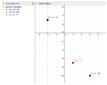
Addition and Subtraction: It starts by defining the numbers that we are going to use for each operation, in this case, the sums will be z1 and z2, and the variable z3 will store the result of the sum [1].
>> z1 = -4+3i;
>> z2 = 6 - 10i;
>> z3 = z1+z2
z3 = 2.0000 - 7.0000i
Graph: In this process, the commands explained above are used to plot all the points of the complex numbers defined and their corresponding result (Fig. 1). Once we entered the following commands in the MATLAB command window, we obtained the graph on the left (Fig 1.)
>> grid on
>>plot(z1,’ob’,’MarkerSize’,7,
’MarkerFaceColor’, ’b’); text(real(z1) + 0.08,
imag(z1), ‘-4+3i’)
>> hold on
>>plot(z2,’ob’,’MarkerSize’,
7,’MarkerFaceColor’, ’b’);
text(real(z2)+0.08,imag(z2),’6-10i’)
>> grid on
>>plot(z3,’or’,’MarkerSize’,
7,’MarkerFaceColor’, ’r’);
text(real(z3)+0.08,imag(z3),’2-7i’)
>> hold on
>> title(‘Add Complex Numbers’)

FIG. 1 Complex Numbers Addition and Multiplication in MATLAB (the sums are shown in blue and the result is red)
The procedure for subtraction is the same.
Multiplication and division: The variables z1 and z2 are multiplied and the result is stored in the z5 variable
>> z5 = z1*z2
z5 =
6.0000 +58.0000i
Graph: To produce the graph, we introduced the following commands and obtained the graph on the right (Fig. 1). The same procedure is performed for division.
>> grid on
>>plot(z1,’ob’,’MarkerSize’,
7,’MarkerFaceColor’,’b’);
text(real(z1)+0.08,imag(z1),’-4+3i’)
>> hold on
>>plot(z2,’ob’,’MarkerSize’,
7,’MarkerFaceColor’,’b’);
text(real(z2)+0.08,imag(z2),’6-10i’)
>> grid on
>> plot(z5,’or’,’MarkerSize’,
7,’MarkerFaceColor’,’r’);
text(real(z5)+0.08,imag(z5), ‘6+58i’)
>> hold on
>> title(‘Complex Numbers Multiplication’)
Module and Conjugate: For this example, we define again z1, this time with the value of z1 = 9 + 13i

Now the module and conjugate is found with the corresponding commands. The result is shown in Fig. 2.
Module
> a = abs(z1)
a =15.8114
Conjugate
>> z1conj = conj(z1)
z1conj =
9.0000 -13.0000i
>> grid on
>>plot(z1,’ob’,’MarkerSize’,
7,’MarkerFaceColor’,’b’); text (real (z1) + 0.08,
imag(z1), ‘9+13i’)
>> hold on
>>plot(z1conj,’og’, ’MarkerSize’, 7,’MarkerFaceColor’,’g’); text(real(z1conj)+ 0.08,imag(z1conj), ‘9- 13i’)
>> hold on
>> title(‘ Complex Numbers Module and Conjugate ‘)

To take into account: It is possible to find as an example the module of several numbers at the same time, inserting them in the form of a matrix as shown below.
>> abs([z1,z2,z3,z4,z5,z6])
ans = 3.6056 7.8102 9.4868 7.6158 28.1603 0.4616
Roots of a complex number: To find the roots of a complex number, we will generate a script (Fig. 3).

clear all
clf
Z=input(' Enter the complex number:'); N=input('Enter the root you want to find out: '); a=abs(Z); b=angle(Z);
plot(Z, 'ob', 'MarkerSize',7, 'MarkerFaceColor', 'b'); text (real (Z) + 0.3, imag(Z)+0.0l, 'Z')
hold on % Keeps the point drawn so it is not erased when drawing other lines
for k=0:(N-l); % this "for" count each one of the roots that will be found.
parameter = (b+2*k*pi)/N; % Parameter to be applied to cos and sin
Roots(k+l) = a
(l/N)* (cos(parameter) + i*sin(parameter))
plot (Roots (k+l), 'ok', 'MarkerSize',3, 'MarkerFaceColor', 'k'); text (real (Roots (k+l)) + 0.l5, imag(Roots (k+l))+0.0l, strcat('R',int2str(k+l)))
% The previous plot graphs the found points of the roots
%strcat Concatenates the text 'R' with the root number
%-----------Example: Rl, R2, R3...
end
%plot(x,y)
plot (Roots, '-b') % The lines of union between points with the appropriate format are plotted
hold on % Necessary for you to hold each line or if they will not be overdrawn
plot([Roots (l), Roots (N)], '-b') % This line joins the start point with the end point to complete the figure
grid on % Draw the graph grid
title (strcat('Roots of a complex number for n=',int2str(N)))
Polar form of a complex number: The polar form of a complex number can be observed using the MATLAB polar command (Fig. 4). For this, we will find the angle and magnitude as follows:
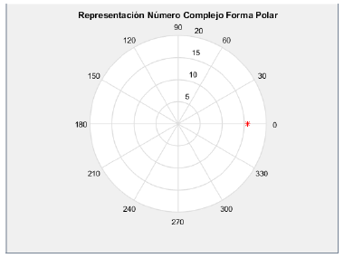
>> magnitude = abs(Zl)
magnitude =
11.2712
>> angle = angle(Z1)
angle =
1.0913
With the results obtained, we used the polar command passing as a the same parameter.
>> polar (angle, magnitude)
>> title ('Polar Representation form of Complex Number')
B. Complex numbers in GeoGebra
In GeoGebra the imaginary part (i) must be written with the command Alt+i to be identified as a complex number [10]. To represent a complex number in the plane, the number is entered in the input bar [11].

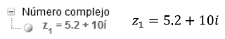
Operations between complex numbers: To perform operations between complex numbers, GeoGebra allows representing them also in the plane [12]. We enter the two or more numbers to be operated and then declare a  as the result of the operation. Results of the multiplication are shown in Fig. 5, and the division in Fig. 6
Addition and Subtraction:
Ex.: Shown in Figure 5.
Multiplication and division:


Module and conjugate: GeoGebra has predefined functions and commands to find the module and the conjugate of a complex number. The module is obtained with the function abs ( ) or with the command longitude [], and the conjugate with the function conjugated^ y) or with the command Refleja[EjeX].
To find the module, we enter the following in the input bar:

To find the conjugate, we enter the following in the input bar:

The value of a corresponds to the module of the number, and z1' corresponds to the conjugate (Fig. 7).

Roots of a complex number: In order to find the root of a complex number in GeoGebra, it is necessary to download an application that is available in the official GeoGebra web page (raices.ggb). After downloading the file, we opened GeoGebra, which comes with a predetermined data in the algebraic view. All values can be modified, but to obtain the result we should simply modify the complex number "A" and the value of "n" (Fig. 8).
Ex.:
Find the roots for n=4 y n=7

For n=4:

Polar form of a complex number: To represent a complex number of polar form (Fig. 9), it is necessary to download an application called complex number polar and trigonometric, which is found in the official webpage of GeoGebra. Once the .ggb file has been downloaded it can be opened in GeoGebra. The program comes with a predetermined data in the algebraic view. All the values can be modified, although to obtain the result, we simply modify the complex number.
Ex.:
Find the polar representation of:

IV. DISCUSSION
MATLAB and GeoGebra are powerful tools with their own and differentiated qualities. The fact that MATLAB uses its own programming language allows it to evolve regarding the way it treats the operations with complex numbers and some other referring subjects. To increase the observance of the virtues that this software tool can offer, it will be possible to develop a small application that performs the same operations shown in this paper automatically with the MATLAB language, in order to improve the graphical properties of the representation of each operating result, resembling more to those shown by GeoGebra, being more user friendly.
V. CONCLUSIONS
Teaching complex numbers can be simplified in some way by using graphical tools that allow anyone to retain the information they want to learn more easily. MATLAB is a very powerful mathematical software that is more oriented toward code operation using its own programming language. GeoGebra is geared more toward usability and a graphical environment. The two tools have special characteristics that make them suitable for teaching complex numbers; all depends on the appropriate choice, depending on the context in which the teaching is taking place.

