1. Introduction

Modal identification techniques estimate the dynamic properties of a structure, such as natural frequencies, mode shapes and modal damping ratios, by measuring its dynamic response. This field has gained significant importance in the last decades because it is an indispensable step for many modal updating techniques (^{Vélez et al., 2009}; ^{Zárate & Caicedo, 2008}), operational modal analysis (^{Ubertini et al., 2013}), human induced vibration analysis (^{Ortiz et al., 2012}), structural health monitoring methods (^{Caicedo & Marulanda, 2011}), structural control (^{Gómez, 2011}; ^{Gómez et al., 2008}) and damage prognosis methods (^{Bartram & Mahadevan, 2014}). Several techniques for the identification of modal properties of structures have been developed and validated in the last thirty years (^{Doebling et al., 1996}; ^{Farrar et al., 2004}). Traditionally, due to physical and economic constraints, only a few degrees of freedom of the total degrees of freedom of the structure are monitored for modal identification. A finite number of sensors are placed at key locations on the structure creating challenges in the identification of the natural or operational mode shapes due to low spatial resolution of the measurements. Only few structures have been densely instrumented such as the Tsing Ma suspension Bridge, the Kap Shui Mun cable-stayed Bridge and the Ting Kau cable-stayed Bridge, in Hong ^{Kong (Ko et al., 2000}). These bridges incorporate a monitoring system with 774 sensors, including strain gauges, accelerometers, displacement sensors, level transducers, anemometers, temperature sensors and weight-in-motion transducers. The Commodore Barry Bridge, in the United States, has nearly 500 static and dynamic transducers operating for monitoring vibrations, local deformations, displacements and ambient conditions, among other variables (^{Li et al., 2004}). An example of one of the world’s most densely instrumented structures is the Guangzhou New TV Tower in Hong Kong, which incorporates 527 sensors in the construction stage and 280 sensors in the in-service monitoring system (^{Ni et al., 2009}; ^{Yi et al., 2012}). Despite the fact that these structures have spatially dense monitoring systems, subsequent analysis (i.e. Modal identification, model updating, damage identification) are still a challenge because the large amount of data collected during testing or operation of the structure.

Mode shape expansion methods are used to calculate spatially dense mode shapes based on the information of discrete points, minimizing the impact of the low spatial resolution of measurements. These techniques can be classified into three main groups according to ^{Levine-West et al. (1994)}: i) spatial interpolation techniques, which use a finite element model geometry to expand the mode shape; ii) properties interpolation techniques, which use the finite element model properties for the expansion; and iii) error minimization techniques, which intend to minimize the error between the expanded and the analytical mode shape using projection methods. Methods in the first group are sensitive to spatial discontinuities, quantity and location of sensors and the mode pairing procedure. The ^{Guyan method (Guyan, 1965)}, which assumes negligible inertial forces at the unmeasured DOF; and the ^{Kidder method (Kidder, 1973)}, which uses the complete dynamic equations to calculate the modal coordinates at the unmeasured DOF, are included in the second group. The Procrustes method (^{Smith & Beattie, 1990}), which uses an orthogonal projection, and the least-squares minimization methods are examples of the third group of modal expansion techniques.

In general, mode shape expansion methods can introduce errors into the modal identification process due to: i) discrepancy between the location of the sensors and the location of DOF in numerical models, ii) measurement errors, and iii) modeling errors (^{Balmes, 2000}; ^{Pascual et al., 2005}). Common solutions to address the discrepancy between the location of sensors and modeled DOF are ignoring distances between the sensor and the numerical DOF, modifying the FE model to match sensor locations, and adding nodes and/or rigid links in the FE model to approximate the location of the sensor. In addition, analytical models are based in assumptions that might not correctly represent the actual structure. These assumptions create modeling errors that introduces inaccuracies from a model reduction and model updating perspective.

This paper proposes the use of a mobile sensor for modal identification in civil infrastructure, improving the spatial density of the identified mode shapes without substantially increasing the number of sensors in the structure (^{Marulanda & Caicedo, 2009}). A fine grid of discrete points representing the operational mode shape is constructed using information of the structures’ motion avoiding the need for modal expansion. Furthermore, the methodology only requires the use of one or few single sensors to calculate highly spatial mode shapes. The proposed methodology is described for one-dimensional systems but it can be easily expanded to two dimensional structures such as shells. In addition, the methodology does not assume any type of model which makes it applicable to any type of structural systems. The methodology is verified numerically using an Euler-Bernoulli beam and it is validated experimentally using a bench-scaled steel beam. A traditional modal identification technique was applied to the experimental beam to obtain baseline results.

2. Methodology

The use of mobile sensors for civil engineering applications opens the door to new possibilities in sensing technology, modal identification, structural health monitoring and damage prognosis. First, standard system identification techniques such as the Stochastic Subspace Identification (SSI) (^{Van Overschee & De Moor, 1996}) are used to determine the natural frequencies of the structure with a sensor parked at a fixed location. Then, the sensor is moved along the structure capturing one record of acceleration. Spatially dense mode shapes are extracted from this single signal. This paper presents the case when the structure is excited with a simple harmonic force at a specific frequency and the sensor moves with a constant velocity.

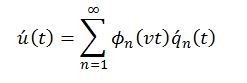
The methodology is applicable to any structural system but for demonstration purposes consider the case of a one-dimensional linear time invariant system under dynamic excitation. If the response of the system is measured with a moving sensor travelling at a constant speed v = x/t, the acceleration response can be written as a function of time only (^{Marulanda & Caicedo, 2009}):

()1

where ( _n (vt) is the n-th natural vibration mode and q´ _n (t) is the acceleration response of the n-th mode in generalized coordinates.

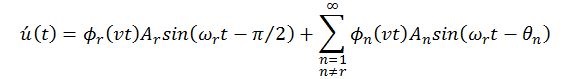
Considering the case where the external force is harmonic and in resonance with the r-th natural mode of vibration, the measured steady state acceleration of the structure can be written as

()2

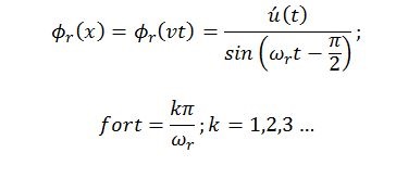
The measured response is an infinite summation of sine functions with the same frequency but different amplitudes and phases. The amplitudes of the sinusoidal terms vary with time due to the mode shape (or with the position of the sensor). For each sinusoidal term different to the r-th mode, the phase (_n is constant and different to (/2. In theory, the identification of the r-th mode could be performed as

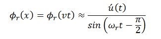(3)

The identification of the mode shapes from Eq. (3) poses two main challenges: i) the influence of the non-resonance modes, and ii) the synchronization between the acceleration record and the sinusoidal function in the denominator of the right hand side of Eq. (3).

At resonance, contributions of the non-resonance modes are not zero. Consider, for example, a uniform simply supported beam, the n−thnatural vibration mode shape and its corresponding natural frequency are

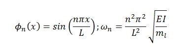(4)

where 𝐿 is the total length of the beam, 𝐸 is the elasticity modulus of the material, 𝐼 is the moment of inertia of the cross section, and 𝑚 𝑙 is its mass per unit length. Assuming L = 60m, E = 25GPa,I, I=6.75m⁴, m_l = 150kN/g/m, (_n = 0.05, the 1^st and 5^th natural frequencies of the structure are 1.45 and 36.24 Hz, respectively.

Figure 1 shows the simulated acceleration responses of a moving sensor at a constant velocity of v = 3 m/s when the structure is excited with a sinusoidal load with a frequency equal to the 1^st and 5^th natural frequencies. The load is applied at the center of the beam with amplitude p_o = 1kN. Ten modes of vibration are used to calculate the response of the beam at x = vt, simulating the sensor moving at a constant velocity.

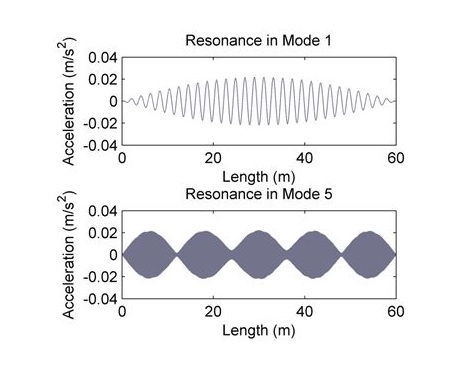
Figure 1 Simulated acceleration measured by the mobile sensor: (a) resonance in mode 1; (b) resonance in mode 5. 

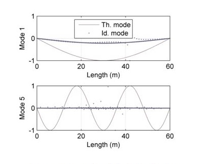
Figure 2 shows the comparison between the 1^st and 5^th identified mode shapes, using Eq. (3), with the corresponding theoretical modes. MAC values (^{Allemang, 2003}) for these modes are 0.990 and 0.009, respectively. Errors in the identification process are due to the influence of the non-resonant modes which can be minimized using only the peak values of the sin(ω _r t - (/2) function in Eq. (3). Therefore the r - th mode can be identified as

()5

Figure 2 Theoretical and identified mode shapes using Eq. (3): (a) 1^st mode; (b) 5^th mode. 

The comparison between the identified 1^st and 5^th mode shapes using Eq. (5), with the corresponding theoretical modes is shown in Figure 3. The velocity of the sensor and the resonance frequency determine the number of points in the modal identification. A total of 57 and 1449 points were obtained for the 1^st and 5^th modes, respectively, with a single 20 seconds acceleration signal sampled at 200 Hz. MAC values of 1.000 and 0.999 were calculated between the 1^st and 5^th identified modes and the theoretical ones. Similar results to those shown in Figure 3 were obtained for the other 8 modes of vibration considered on the simulation.

Figure 3 Theoretical and identified mode shapes using Eq. (5): (a) 1^st mode; (b) 5^th mode. 

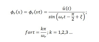
The phase ( between the acceleration record and the sinusoidal function in the denominator of Eq (3) will be present in experimental tests and include errors in the identification. Including this phase in Eq (5) we obtain

( 6)

Figure 4 MAC values as function of ξ: (a) resonance in mode 1; (b) resonance in mode 5. 

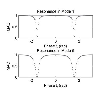
Figure 4 shows the MAC values between the identified and the theoretical mode shape for different values of (. The range of acceptable phase ( changes with the identified mode. Higher modes of vibration are more sensitive to this parameter. The influence of the phase lag ( can be minimized by synchronizing the acceleration record such that the maximum accelerations correspond to the values of 𝑡 on Eq. (5). In other words, having a value of ( close to zero.

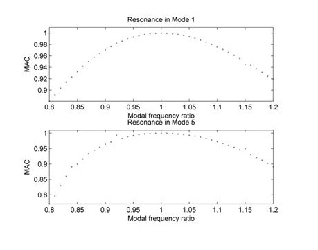
The first step for the use of the proposed methodology in a full scale implementation would be the identification of the natural frequencies using a standard identification procedure. As in that case will be uncertainty in the identified frequencies, Figure 5 shows the MAC value between the identified and the theoretical mode shapes when the identified natural frequencies vary from 0.80 to 1.20 of their actual value. In each case, the variable frequency is used as the forcing frequency and the resonant frequency for the mode shape identification. As can be seen, the methodology is robust to uncertainties of around 10 and 5% in the initial identification of the natural frequencies of the 1^st and 5^th modes, respectively. These values of uncertainty are considered acceptable. ^{Giraldo et al. (2009)} use an acceptable 2% threshold for the identified natural frequencies in an automated identification process with experimental data. The authors report average errors in the natural frequencies under 0.1% using different standard identification techniques.

Figure 5 MAC values for variations in the identified natural frequencies: (a) resonance in mode 1; (b) resonance in mode 5. 

3. Results and discussion

A 15.24 cm × 0.32 cm × 121.92 cm (6 in × 1/8 in × 48 in) simply supported steel beam was used for the experimental validation of the proposed methodology. A detailed traditional modal identification procedure was performed to identify the dynamic behavior of the beam and compare the results with results from the proposed methodology.

Three capacitive PCB 3701D1FA20G accelerometers were used to measure the vibration of the beam, each one with a PCB 478A01 signal conditioner. The accelerometers have a sensitivity of 100 mV/g (± 5 %), a range of ± 20 g, and a frequency range from 0 to 300 Hz (± 5 %). The signal conditioner powers the sensor, compensate for the nominal DC offset and the offset due to the effect of gravity and send the signal to the acquisition system. To transform the continuous signal to digital format a Measurement Computing USB-1208LS module was used. The USB module has a resolution of 12 bits in differential mode, a maximum sampling rate of 1.2 kHz in continuous scan mode and a variable input range from ± 1 to ± 20 Volts. The acquisition module sends the signal of up to four channels (in differential mode) in digital format to a laptop computer to be recorded using a Measurement Computing’s software.

3.1 Traditional modal identification

The natural frequencies and mode shapes of the beam were obtained using the Stochastic Subspace Identification (SSI) method (^{Van Overschee & De Moor, 1996}). The algorithm calculates the dynamic properties of the system (i.e. natural frequencies, mode shapes and damping ratios) from a state space representation. SSI has proven to be a reliable and simple tool (^{Giraldo et al., 2009}), and is used in this work to identify mode shapes for the experimental verification.

Impact excitation tests using a PCB 086C03 general purpose modal analysis impact hammer were performed to identify the first two natural frequencies of the beam. The hammer has a mass of 0.16 kg, a sensitivity of 2.25 mV/N (± 15 %), and a range of ± 2200 N. A reference accelerometer was located at 32 inches from one end of the beam while the other two sensors were moved throughout the beam at two inches intervals. Five impact tests of one minute length, using a combination of short and long intervals between hits, were performed for each testing location using a sampling frequency of 400 Hz. Mean values and standard deviations of the first two natural frequencies were calculated using the SSI method. The mean value of the first natural frequency is 4.681 Hz with a standard deviation of 0.018 Hz. The mean value of the second natural frequency is 18.862 Hz with a standard deviation of 0.171 Hz.

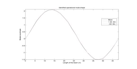
A Brüel & Kjær vibration exciter type 4809, located at 12 inches from the left support, was used to identify the operational mode shapes of the beam. The beam was excited with the actuator tuned at a constant forcing frequency of 18.8 Hz, controlled by a Quanser Q8 data acquisition and control board, and a Brüel & Kjær power amplifier. The reference accelerometer was kept at 32 inches from the left support of the beam while the other two sensors were moved throughout the beam at two inches intervals. Five tests of 30 seconds length were performed for each testing location using a sampling frequency of 400 Hz. Mean values and standard deviations of the modal coordinates of the operational mode shape with the actuator tuned at 18.8 Hz were calculated using the SSI method, and are shown in Figure 6.

Figure 6 Identified operational mode shape using the SSI. 

3.2 Experimental implementation

The proposed methodology was experimentally implemented with the previously described setup, using a small cart with a constant speed motor (Figure 7). An accelerometer was attached to the cart and the cart was displaced from one end of the beam to the other. The vibration exciter, located at 12 inches from the left support, was tuned to apply a constant frequency harmonic force at 18.8 Hz. The cart was reinforced with an aluminum plate to reduce local vibrations. Four magnetic wheels with 2.395 inches of diameter and 0.25 inches of thickness were used to avoid the cart jumping. Figure 8 shows the acceleration of the moving sensor using a sampling frequency of 400 Hz.

Figure 7 Experimental setup (^{Marulanda & Caicedo, 2009}). 

Figure 8 Acceleration time history recorded with the mobile sensor. 

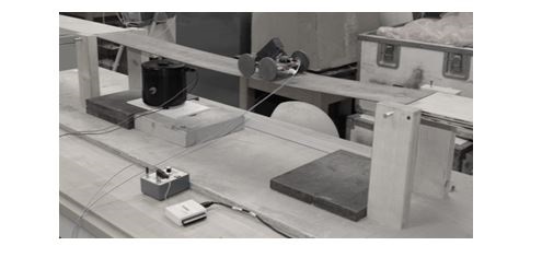
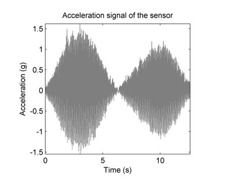
Figure 9 shows the identified operational mode shape using the proposed methodology. A total of 32 points were obtained for constructing the identified mode with a single 12.6 seconds signal. A MAC value of 0.969 was obtained between the operational mode shape identified using the standard approach (SSI) and the one using the methodology. Differences between the mode shapes are mostly in the right half of the mode because the mass of the cart is modifying the system dynamics. A smaller effect was found close to the actuator. The weight per unit length of the beam is 0.210 pounds per inch and the weight of the car is 1.209 pounds, distributed in the front and rear axis which are separated by 2.5 inches.

Figure 9 Identified operational mode shape using the proposed methodology. 

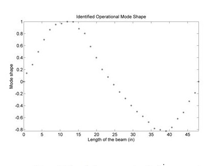
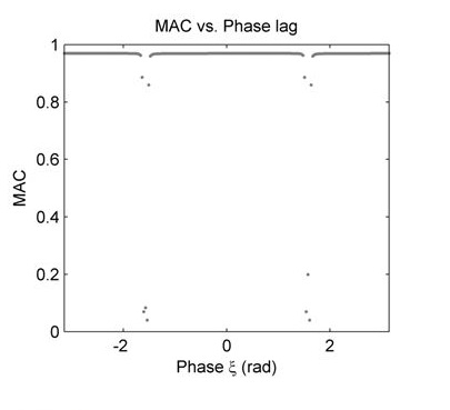
Figure 10 shows the MAC value between the operational mode shape identified using the standard approach and the one using the methodology for different values of 𝜉 (Eq. (6)). The experimental results have good agreement with the numerical simulations results shown in Figure 4.

Figure 10 MAC values as function of the phase lag in the experimental implementation 

4. Conclusions

A methodology for the identification of mode shapes of a dynamical system under harmonic excitation using mobile sensors was proposed and verified using numerical and experimental data. The methodology minimizes errors in the identification process due to the influence of the non-resonant modes and it is robust to uncertainties in the initial identification of the natural frequencies. In the proposed numerical example, the methodology was robust to uncertainties of around 10 and 5% for the 1st and 5th modes, respectively. An important issue in the experimental implementation of the methodology is the synchronization of the acceleration record and the sinusoidal function to minimize the effect of the phase lag.

The number of points in the modal identification depends on the velocity of the sensor and the frequency of the identified mode. In this particular case, from 57 to 1449 points were obtained with a single 20 seconds simulated signal. MAC values of 1.000 and 0.999 were obtained for the first and fifth mode, respectively. Similar results were obtained for the other 8 modes of vibration considered on the simulation.

A simply supported steel beam was used for experimental validation. A detailed standard modal identification procedure was performed to identify the dynamic behavior of the beam and compare the results with results from the proposed methodology. A total of 32 points were obtained for constructing the identified mode with a single 12.6 seconds signal. A MAC value of 0.969 was obtained between the operational mode shape identified using the standard approach and the one using the proposed methodology. Differences between the two identified mode shapes are mostly due to the influence of the mass of the cart over the beam. This is not expected in full-scale implementations on civil structures.