


 English (pdf)
 Article in xml format
 Article references
 Send this article by e-mail
 Cited by SciELO
  Cited by Google
  Similars in
SciELO
Similars in
SciELO  Similars in Google
 Permalink
INTRODUCTION
Graphene is a 2D system formed by six carbon atoms in a hexagonal or honeycomb lattice [1-2]. This translational symmetry creates conduction and a valence band that touches each other in six points known as Dirac points where the dispersion is linear, and the charge carriers behave as massless Dirac Fermions [2-5].
Today, graphene is produced in macroscopic quantities to design new electronic devices [6]. However, the increase in size brings electrical, thermal, and mechanical performance [6-7].In particular, the high-quality electrical properties of graphene are affected by the formation of edges. Edge states are known to play an essential role in the quantum Hall regime [8-9]. For graphene, particularly, it was shown by scanning tunneling microscopy and spectroscopy that the quantum Hall edge states display confinement characteristics by an atomically sharp edge, without edge-state reconstruction [10].
Here, we use a tight-binding approach to investigate the localization properties of quantum Hall edge states from graphene flakes with edges. To establish how the charge is distributed along the edge or bulk and how the current potentially flow along the nanostructure, we use the recursive Green’s function method [1, 11-12] to study, numerically, the transmission, the charge and current density originating from the electron scattering through of monolayer graphene.
1. NUMERICAL MODEL
We consider monolayer graphene with M atoms in the armchair direction and N atoms in the zig-zag direction, as shown in figure 1. In this way, the dimensions of the lattices in x (Lx) and y (Ly) directions are given by equations (1) and (2):
 (1)
(1)
and
 (2)
(2)

Source: own elaboration.
Figure 1 Schematic representation of monolayer graphene lattice with NxM sites in the presence of a magnetic field. The graphene is connected to two semi-infinite electrodes: source (S) and drain (D)
where a=1.42 ˚A is the lattice constant for graphene per unit cell. The tight-binding Hamiltonian to first neighbors is given by equation (3):
 (3)
(3)
where c i (c i †) annihilates (creates) an electron at site I and the sum j runs over neighbor sites, ϵ i is the effective orbital energy of a carbon atom. The external magnetic field B, perpendicular to the graphene sheet of area A, is introduced using the phase ∅ ij in the hopping parameter t=2.7 eV along the ∓ y -direction, as shown in equation (4):
 (4)
(4)
Where the magnetic flux  is calculated through the equation (5):
 (5)
(5)
We consider disorde (W) through on-site white-noise fluctuations by sorting uncorrelated orbital energies within ϵi ≤ W/2. We focus the analysis on the lowest Landau levels [13] for small magnetic flux  , a value where the lattice effects on the electronic spectra (Landau levels) are negligible.
For these calculations, coherent transport across grain boundaries in graphene is studied within the Landauer-Buttiker formalism [14], which relates the conductance G(E) at a given energy E to the transmission probability T(E) between the contacts using Equation (6):
 (6)
(6)
Where  is the conductance quantum. T(E) is evaluated in equation (7) employing the recursive Green’s function approach using two-terminal device configurations with contacts represented by the semi-infinite ideal graphene leads:
 (7)
(7)
Where G S is the retarded Green’s function of the system, which can be found from [15] as shown in equation (8):
 (8)
(8)
In these expressions, H S is the Hamiltonian for the scattering region, E´ is the energy and Σ L(R) is the self-energy that couples the scattering region to the leads, which can be calculated from Green’s function gL(R) as shown in equation (9):
 (9)
(9)
The broadening function Γ L(R) in equation (7) are also obtained numerically using a recursive technique [16] and determined from the equation (10):
 (10)
(10)
Charge and current are intimately related through the continuity equation (11):
 (11)
(11)
where  is the bond charge current operator thatresults from the difference of electrons flow in opposite directions, in this lattice version,
  is given by equation (12):
 (12)
(12)
The connection with the Green’s function arises because the quantum statistical average of the bond charge current operator of the form (c † n c n ) are related to the lesser Green’s function G < (E) [17] in equation (13):
 (13)
(13)
where I 0=2e/h = 77.48092 μA/eV is the natural unit of bond charge current density. The lesser Green’s function in the absence of interactions can be resolved exactly as shown in equation (14):
 (14)
(14)
where fL(R) is the Fermi distribution of the left(right)contact and t nn´ is the hopping parameter between sites n’ and n. To quantify the electron flow in a layer, we defined the layer current density through the equation (15):
 (15)
(15)
Here, k represents a site in the central region of the nanoribbon. Equation (16) define the total current at site, k is calculated adding the current bond equation (15) between site k and its neighboring sites n:
 (16)
(16)
Once again, since we are working on a pristine nanoribbon, the current density in any slide of our device is the same; because of that, we associated it with a layer current density in equation (16). Complementary to current density, charge density at site k can also be expressed using the lesser Green’s function in equation (17):
 (17)
(17)
At equilibrium, all states are occupied as specified by the Fermi-Dirac distribution (f (E)), and the lesser Green’s function acquires the simple form defined in equation (18):
 (18)
(18)
where A(E) is the spectral function determined from the equation (19):
 (19)
(19)
which is related to the local density of states (LDOS) at r position using equation (20):
 (20)
(20)
It is noteworthy that at low bias and low-temperature ρc is given by equation (21):
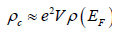 (21)
(21)
that charge density (ρc) has the same local distribution of LDOS (ρ). We are interested in how are charge and current distributions related, with no loss of generality, to keep explanations and figures as simple as possible, we will refer to LDOS as charge distribution. The density of states DOS can be calculated from the LDOS through equation (22):
 (22)
(22)
3. RESULTS AND DISCUSSION
In monolayer graphene without a magnetic field, the transmission probability in the linear regime shows steps that can be understood from the energy dispersion relation of graphene infinite ribbons [18], namely, the dimensionless conductance Go is given by the number of bands crossing the Fermi energy E.
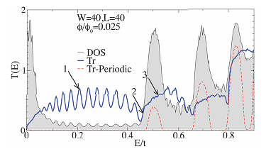
Figure 2 shows the density of states DOS and the transmission probability as a function of energy for square-shaped monolayer graphene, with 40 atoms in the armchair direction and 40 atoms in the zig-zag direction, in the presence of a perpendicular magnetic field B (we considered a magnetic flux  and connected to two unidimensional electrodes (see figure 1).With periodic boundary conditions, the system breaks into Landau levels [19] that, for a periodic graphene layer, have energies given by equation (23):
 (23)
(23)
where j = 0, 1, ... labels the Landau levels and the cyclotron frequency ω is given inequation (24):
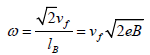 (24)
(24)
where vf=106 m/s is the Fermi velocity for graphene and lB is the magnetic length.
Source: own elaboration.
Figure 2 (Black line) charge density (DOS) and transmission probability T(E) for monolayer graphene system with (red line) and without (blue line) periodic boundary conditions. Both systems are considered with 40x40 atoms and a magnetic flux of 
To monolayer graphene with (red line) and without (blue line) periodic boundary conditions, we consider on-site white-noise disorder with W/t = 0.4. The Landau Levels degeneracy is broken in both cases, forming a broadened resonance in transmission probability at Landau energies given by equation 9, as shown in the figure. 2. On the other hand, to a system without periodic boundary conditions, the DOS (black line) shows an oscillatory behavior as a function of energy between Landau levels. It should be noticed that the DOS shows the same resonances as the periodic case at the landau energies. From a comparison between the resonances in the transmission spectrum of a system, with and without edges, periodic and no periodic monolayer graphene, respectively, one can suggest that the position of the Landau bands are very similar for both systems. Therefore, broadened Landau states do not change with the edges shape.
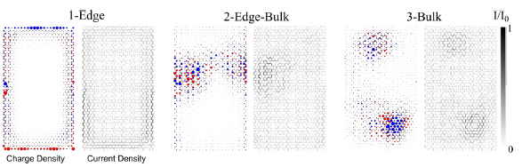
Figure 3 plotted the charge (left panel) and current (right panel) spatial density for three electronic states of monolayer graphene without periodic boundary conditions. The diameters of the depicted red and blue circles are proportional to the wave function amplitude over each atomic site of the lattice given by the LDOS. The headed arrows show the current direction between two neighbors, clarifying the relation between the charge and current.
Source: own elaboration.
Figure 3 Spatial distribution of charge densities and current densities over graphene nanoribbons with zig-zag and armchair edges. (1), (2) and (3) corresponding to the energies indicated by the numbered arrows in figure 2
The three electronic states in figure 3: 1-Edge, 2-Edge-bulk and 3-bulk, correspond to the arrows (1, 2, 3) on the transmission spectrum shown in figure 2. To states with energies between the j=0 and j=1 Landau levels (arrow 1), the magnetic length is l B =0.58nm at the magnetic flux considered, which means that the system size L=16 nm is larger than magnetic length (L>>l B ). Therefore, the 1-Edge has higher charge density localization on zig-zag and armchair edges. It is appreciated that current is homogeneously distributed over edge layer while is nearly zero over bulk layer.
The electronic states in the intermediary region (arrows 2) are characterized by a charge density distributed on the edges and the bulk with a low transmission probability. We can understand that the charge is completely localized on one of the two sites of the unit cell in the edges; electrons on these sites cannot jump on their nearest neighbors, causing no electron flow over the edges. In the central region of each Landau level (arrows 3), we have the smallest charge density values on the edge. This result is coherent with bulk extended states; the current density is homogeneously distributed over bulk, allowing electron hopping among sites. This is related to the higher complexity and localization length of the quantum Hall states for the higher Landau Levels index.
2. CONCLUSIONS
The T(E) and DOS presented here are a numerical tool that allows a more detailed observation of the differences between monolayer graphene with and without periodic boundary conditions (see figure. 2). The charge and current density of an electronic state depend on their energy proximity to the Landau levels. We have identified energy ranges between adjacent Landau levels for which the transmission probability and DOS are oscillatory functions, and the charge and current density of different states are distributed on the edges.
One can see that the shape and position of the resonances in T(E), for both systems (with (blue line) and without (red line) periodic boundary conditions are in relation with the Landau bands. Therefore, broadened Landau bands are robust effects. In monolayer graphene, without periodic conditions in the presence of a perpendicular magnetic field, it is possible to find states with a charge and current density localized preferentially between the bulk and the edges. This behavior appears from a different mechanism as a reminiscence of the case with edges with a magnetic field where the charge and current density circulate all over the edges.

