


 Inglés (pdf)
 Articulo en XML
 Referencias del artículo
 Enviar articulo por email
 Citado por SciELO
  Citado por Google
  Similares en
SciELO
Similares en
SciELO  Similares en Google
 Permalink
Introduction
The dissolution phenomenon plays an important role in several industrial and biological processes such as drug delivery via mucosal surfaces (Jug et al., 2018), water treatment (Pham, Sedlak and Doyle, 2012), or controlled release of inhibitors from coatings (Pham et al., 2012), among others. Once a solute is introduced in a solvent, it is expected to engage in a dynamical process where the solute particles migrate from the highest to the lowest concentration regions. This phenomenon is strongly dependent on thermodynamic variables such as pressure, temperature, and the nature of the solvent.
From a mathematical point of view, the dissolution rate can be accounted for by using the Noyes-Whitney equation: (Noyes and Whitney, 1897)

where m is the solid mass at a given time t, S is the solid surface area, h is the diffusion layer thickness, C s is the solute solubility, C t is the solute concentration at a time t, and D is the diffusion coefficient. It is known that the diffusion coefficient characterizes the ease with which each particle moves into a given solute and depends on many factors such as the size and shape of the solute, solvent viscosity, and temperature.
If a solute with a spherical geometry is considered, it is possible to see that the integration of Equation (1) results in the Hixson-Crowell model (Hixson and Crowell, 1931). Details about the procedure can be found in the literature (Beauchamp, 2001; Hixson and Crowell, 1931; Hixson and Baum, 1942).

where k represents the constant kinetic of dissolution given by

It can be observed that k depends on density (p), diffusivity (D), and solubility parameters (Cs). k is also explicitly dependent on temperature through an Arrhenius-like law given by the following Equation:
where A is the pre-exponential factor, E a is the activation energy, R is the ideal gas constant, and T is the temperature.
Although the dissolution constants of spherical solids have been previously reported, to the best of our knowledge, the effect of the agitator geometry on it has not yet been considered. This effect is of great importance to understand the dissolution dynamics in stirred tanks where additional variables need to be considered, such as the type of impeller device and the proportions of the tank, deflectors, and agitators (Mc Cabe et al,. 2007). Previous works have been carried out on the effect of different impeller features on different processes. For instance, (Mangwandi et al., 2010) showed that, for a high-shear granulator, impeller speed has an effect on granule size distribution, as well as on structure and shape, which in turn affects the dissolution rate measured by means of the time a certain percentage of granules takes to dissolve. (Legendre et al., 2016) simulated bubble dissolution in a fluid tower to optimize the process of C02 mineralization. Using a specific impeller geometry, they calculated the Hatta number, demonstrating that the effect of the chemical reaction is minimal in contrast to the mass transfer process, as well as presenting the dissolution of mass over time. Kravtchenko et al. (1999) studied the dissolution of food hydro-colloids, for which they empirically found a certain configuration between stirrer and container in order to overcome the issue with lump formation. They were able to quantify dissolution kinetics by assessing the mass dissolved over time. (Jirout et al,. 2011) showed that mixing system aspect ratios have an effect on the mixing of suspensions calculated through the Froud number and dimensionless power consumption necessary for off-bottom particle suspension. (Thakur et al., 2004) demonstrated that, in complex fluids (Newtonian and non-Newtonian), the column-to-impeller distance has an effect on mixing, which was evidenced by means of computing the effective shear rate and the power consumption. (Akrap et al., 2012) studied the effect of variation in the ratio of the impeller diameter to tank diameter, on the nucleation rate of borax decahydrate and crystal growth, but they did not examine dissolution. (Abreu-Lopez et al., 2017) numerically computed the effect of different impeller designs in a batch reactor for aluminum degassing, estimating pressure fields and dimensionless oxygen concentration with respect to time. (Alok et al., 2014) analyzed the effect of different kinds of impeller on mixing in an aerobic stirred tank fermenter, determining the volumetric mass transfer coefficient. They reported a particular kind of impeller to be the most efficient in regards to mass transfer in comparison with the others by measuring the turbulent dissipation rate, which, according to the authors, represents the volumetric mass transfer rate. (Ćosić et al., 2016) studied the influence of the impeller blade angle on the crystallization kinetics of borax. Some of the findings were that the flow pattern of the liquid charge changes significantly with the blade angle, the rate of nucleation increases as the blade angle decreases, and increasing the impeller blade angle significantly impacts the crystal growth rate constant. By means of electrical resistance tompgraphy and computational fluid dynamics, (Kazemzadeh et al, 2020) analyzed the effect of impeller type on the mixing of highly concentrated large-particle slurries. Using three types of axial impellers, they found that the impeller type has impact on the homogeneity of the mixture, the average particle velocity along the tank, and the energy dissipation, which therefore affects power consumption. (Gu et al., 2020) studied floating particle drawdown and dispersion in a stirred tank with four pitched-blade impellers using computational fluid dynamics simulation. The type of impeller can reduce the power consumption at the same impeller speed, and it can also enhance the solid integrated velocity and the level of homogeneity for the floating particle dispersion process under constant power consumption. (Liu et al., 2021) investigated gas-liquid mass transfer and power consumption in jet-flow high-shear mixers. They found that gas-liquid mass transfer performance and power consumption are significantly affected by structural parameters, among them rotor blade angle and rotor blade arc. They also found the gas-liquid mass transfer performance is improved with increasing blade angle and that power consumption is reduced by decreasing the blade angle.
This work aims to experimentally study the effect of impeller geometry on the dissolution rate of spherical candy. In order to do that, the dissolution constant rate will be evaluated considering variations in the geometry of the stirrers, their agitation angular frequency, and the solvent temperature. The activation energy of the dissolution is determined, as well as the pre-exponential factors for every agitator.
Experimental development
Inside a mixing cylindrical tank, it is possible to distinguish three velocity components: the radial component, which acts perpendicularly to the stirrer axis; the longitudinal component, which acts parallel to the axis; and the rotational component, which acts tangentially to the circular trajectory around the axis.
Impellers can be divided into two types: those which generate currents parallel to the axis, called axial flow impellers; and those which generate currents in the radial or tangential direction, called radial flow impellers. The main impeller types for liquids are propellers, paddles, and turbines (Mc Cabe et al., 2007).
In this work, three different impellers were used to generate diverse flow patterns inside the system and observe the effect of different geometries on the dissolution process. The types of conventional agitators used were:
• Agitator 1: This agitator is a paddle which consists of two blades (Figure 1); it mainly produces radial and tangential flow currents, as well as intense shear stresses.

Source: Authors
Figure 1 Agitator 1: paddle agitator, two blades; agitator 2: turbine agitator, four inclined blades; agitator 3: turbine agitator, six disk straightblades
• Agitator 2: This agitator is a turbine type whichconsists of four blades (Figure 1) pitched at 45 ° . It produces both axial and radial flow, as well as high shear stresses.
• Agitator 3: This agitator is also a turbine type which consists of six straight blades (Figure 1). It produces radial and tangential flow, as well as a higher shear stress than agitator 2.
Empirical geometric proportions of the tank and agitator, which are illustrated in Figure 2, were taken into account for the paddle-type and turbine-type agitators shown in Table 1, where D a is the propeller diameter, D t is the water tank diameter, W is the width of the propeller blade, H is the water tank height, and E is the height of the propeller with respect to the water tank bottom. Dimensions were measured using a caliper with an error of ±.


A sketch of the experimental set-up is shown in Figure 3. It consisted of a 1 000 ml beaker filled with 700 ml of water and a candy sphere (solute) immersed in it. The agitation was provided by means of an agitator coupled to a DC motor, whose angular frequency (ω) was controlled using a variable DC voltage source. The rotational speed was practically achieved as soon as the motor is started. Therefore, by changing ω, modifications of the flow pattern inside the tank were obtained.

The spherical mass was initially measured using a precision digital balance (OHAUS) with an accuracy of 0,01 g. Averaging ten candies, the initial mass of the candy was 10,01 g ± 0,49 g. Although the radius was not used, the candy spheres had an average diameter of 17,07 mm ± 0,25 mm. The solid was introduced into the beaker, and the solution was stirred for 2 min under a fixed voltage applied to the motor, which corresponds to a given angular velocity. Afterwards, the candy sphere was taken out and dried. Then, its mass was measured again. This process was repeated 10 times in 2 min intervals at room temperature (20 °C). Time was measured using a digital chronometer with an accuracy of 0,01 s. Five variations in the stirring frequency were chosen for each agitator. The described procedure was performed for the three types of agitators illustrated in Figure 1. Each measurement was repeated five times with different candies. It is important to clarify that, while the agitation occurred, there were no collisions between the candy spheres and the agitator paddles, and no changes in their spherical shape were observed. The candy was introduced and taken out with a strainer in a very short time with the agitator at rest, and it was put on a napkin so water was absorbed the mass was measured, which is why measurement errors in this regard were not significant.
As a second stage of the study, the experimental setup was placed inside a thermal bath under a controlled temperature (Thermo HAAKE Phoenix II circulator). The voltage applied to the motor was kept at 7 V (632 rpm) 0,1 V, and temperature variations between 20 and 70 1°C were implemented and measured with a mercury thermometer. Because the solid dissolution rate and mass loss increased at higher temperatures, it was necessary to take mass measurements more often during this stage (they were taken every minute).
The angular velocity of the agitator was controlled by the voltage applied to the motor and measured using a tachometer with an accuracy of 0,1 rpm. The motor calibration curve is shown in Figure 4, which evidences a direct relation between the voltage applied to the motor and the rotational speed. The results were very similar for the different agitators coupled to the motor because all of them have a small moment of inertia. Numerical values of the calibration curve can be consulted in the Supplementary Information section.
Results and discussion
Dissolution constants at room temperature
For Figures 4 to 11, dots represent the average of five measurements, and error bars are not included since they are smaller than the symbol size.

Figure 5 represents the cube root of mass as a function of time and at room temperature. Dots correspond to experimental points and lines to a linear fit. Although several angular frequencies were considered, for this Figure only, the lowest and the highest angular frequencies are shown for every agitator.
Source: Authors
Figure 5 Cube root solid mass as a function of time for several angular frequencies of the three agitators
It can be observed that, at all frequencies, the three types of agitators follow a linear relation between the cube root of mass and time, which agrees with the Hixson-Crowell model. From the slope of these curves, and considering Equation (2), it was possible to determine the value of the dissolution constant k.
The relation between the angular frequency c of the agitators and the solid dissolution constant k is represented by Figure 6.

Source: Authors
Figure 6 Solid dissolution constant as a function of the angular frequency for the three agitators
Note how, for ω ≤ 632 rpm, the value of k increases. For agitator 1, the difference between the two first dissolution constant values is so small (around 3%) that we can assume that the k remained constant. However, for higher values of co, a decrease with respect to the maximum achieved dissolution constant is found, which is a characteristic of the three types of agitators. This behavior can be attributed to the fact that, for ω > 650 rpm, vortex and high turbulence inside the beaker were experimentally observed, especially for agitator 3, which showed the highest drop in k. The combination of these effects could make the mass transfer between solute and solvent difficult and therefore produce a decrease in mass transfer during the diffusion process. From Figure 6, it is also possible to infer how, for ω < 632 rpm, the higher values of dissolution constants are obtained with agitator 2, which is the one that actually has its blades pitched, thus allowing an axial flow. For ω > 632 rpm, agitator 1 attains the highest rates of dissolution, presumably since it is the one which reported the least of turbulence. This led us to infer that the dissolution constant depends indeed on the geometry used in the agitation system.
Dissolution constants under different temperatures
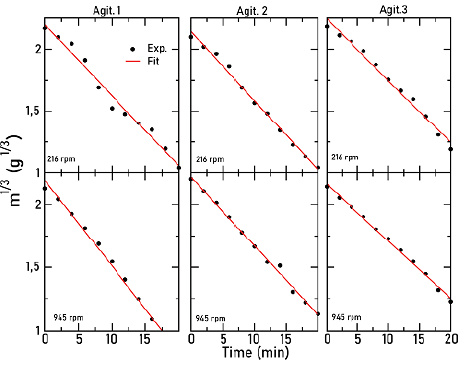
Figures 7, 8, and 9 show the cube root of mass as a function of time for agitators 1, 2, and 3, respectively, for different temperatures as indicated in each Figure. Lines correspond to the fit to the experimental points. In all cases, the angular frequency was held at 632 rpm.

Source: Authors
Figure 7 Cube root of mass as a function of time for agitator 1 at different temperatures, ω = 632 rpm

Source: Authors
Figure 8 Cube root of mass as a function of time for agitator 2 at different temperatures, ω = 632 rpm

Source: Authors
Figure 9 Cube root of mass as a function of time for agitator 3 at different temperatures, ω = 632 rpm
In these Figures, it is observed how, as the temperature increases, there is an increase in the slope absolute value and therefore in the solid dissolution constant. This was expected, since, when temperature increases, there is also an increase in the solubility of particles.
Figure 10 shows the dependence of the solid dissolution constant as a function of temperature for the different agitators used in this experiment. As predicted by Equation (4), there is an increase in the solid dissolution constant as the temperature increases. It is also possible to observe that the dissolution constant is remarkably dependent on the type of agitator, and it is again the agitator 2 which attains the highest dissolution constants for all temperatures. For the highest temperature studied, the difference between the constants decreases, possibly due to the effect of temperature, which exerts a greater influence on the dissolution process than the agitator geometry. Still, agitator 2 keeps attaining the highest constant. Therefore, taking into consideration the results shown in Figure 6, we can say that agitator 2, which produces both axial and radial flow, also induces the highest solid dissolution constants.

Activation energies
Activation energies E a for the dissolution process are determined by taking the natural logarithm of Equation (4), so that

Figure 11 shows the natural logarithm of the solid dissolution constant as a function of the inverse of the temperature for the three types of agitators used in this work. In this Figure, it is possible to observe how every straight line has approximately the same slope (Table 2). Differences between them are about 6% at most. Therefore, it is possible to conclude that the activation energy is approximately the same for all cases and is independent of the agitator geometry. This activation energy is similar to the 23 kJ/ mol value reported by (Beauchamp, 2001). However, in Table 3, which summarizes the pre-exponential factors (A), some remarkable variations appear, since line intercepts in Figure 11 are different in each situation.

Source: Authors
Figure 11 Relation between logarithm of dissolution constant, for all the agitators, and the inverse of temperature
This leads us to conclude that the agitation phenomenon is modified specifically in the pre-exponential factor of the dissolution constant, while the activation energy of the process remains practically constant.


Conclusions
Hixson-Crowell model appropriately predicts the kinetics of the dissolution of solids with spherical geometry. By using this model, it was possible to determine both the kinetic constants and activation energy necessary in the dissolution process. Additionally, the results showed that the agitation rate and agitator geometries affect the kinetic dissolution constant. Therefore, it is important to consider these variables when conducting a dissolution experiment.
Values of the solid dissolution constant are affected at constant temperature by the angular frequency of the agitator in all the studied geometries. The highest values in the constants were obtained for the turbine- type agitator 2, which produces axial and radial flow. However, for higher angular frequency values, the constant decreases, which can be explained in terms of the high turbulence manifested in the formation of vortices.
The activation energy was approximately the same for the three types of agitators used, regardless of their geometry. For the pre-exponential factors, a remarkable difference appeared among the agitators, which leads us to conclude that the geometry of the agitator can affect the kinetic constant specifically in the pre-exponential factor.

