


 Inglés (pdf)
 Articulo en XML
 Referencias del artículo
 Enviar articulo por email
 Citado por SciELO
  Citado por Google
  Similares en
SciELO
Similares en
SciELO  Similares en Google
 Permalink
1. Introduction
Traditionally, the concept of a pedal curve is associated with minimum distance, and thus with orthogonality. For any n-dimensional space (e.g., in ℝ3, see Fig. 1a) given a hypersurface C and a fixed point P (named pedal point), the pedal hypersurface S is defined as the locus of points Q of the minimum distance between the pedal point P and every hyperplane tangent to C [1].
Minimal distance, associated with a Euclidean norm, is intrinsically linked to the concept of perpendicularity. The traditional definition of a pedal curve in two-dimensional spaces is derived from this, as illustrated in Fig. 1b. Thus, the pedal curve of another curve C with respect to a point P, called the pedal point, is defined as the locus of the foot of the perpendicular from P to a variable tangent to C [2,3].
As shown in Fig. 1c, this concept is susceptible to generalization, only in ℝ2, to any angularity condition [4], that is, to any given angle different from 90º. Applying this generalization, we can obtain a family of curves of the same category related by rotation and homothety.

Source: The authors.
Figure 1 Pedal generation concept in three dimensions (a), in two dimensions (b), and the generalization of the concept to any angle (c).
The limaçon of Pascal is a curve that emerges from the application of the pedal concept to a circle [2]. It is possible to use the generalization of the pedal curve to describe a different method to generate a limaçon of Pascal that, to the best of our knowledge, is not described in the literature. This definition can be seen as a singular case of the locus generation method proposed as a problem first in [5] (with some inaccuracies), and described in further detail in [6,7].
1.1 Types of Limaçons
The traditional classification of a limaçon is based on its morphology. The different types are looped, with a cusp (cardioid), dimpled, flat, and convex. However, for the purposes of our discussion, a different classification is more convenient.
As is known, the limaçon of Pascal is the inverse of a conic, when the center of inversion is one of the foci of that conic [8]. It is easy to check it using the polar equation (eq. 1) of a conic with a focus as a pole:
where e is the eccentricity of the conic, and d is the distance to the directrix.
The inverse of this curve with regard to the origin, which, as previously mentioned, is one of the foci of the conic, will fulfill the inversion statement.
 .Solving for r (eq. 2), we obtain the polar equation r=b+a cos(θ)of the limaçon.

Depending on the type of conic, owing to its eccentricity, we obtain a different type of limaçon. It is easy to check, if we consider the ratio b/a in eq. (2), which is
 Therefore, we can classify them as shown in Table 1.
Table 1 Types of limaçon according to the eccentricity of the conic to which it is inverse.

Source: The authors.
According to this definition, we can distinguish three types of limaçons: elliptical (Fig. 2a), parabolic (Fig. 2b), and hyperbolic (Fig. 2c). This nomenclature is used in the remainder of this paper. Note that the focus that serves as the center of inversion is a point of importance in all three types of limaçons.

2. Generalization of the pedal concept in bidimensional spaces
As mentioned in Section 1, in ℝ2 spaces, the pedal curve of curve C is traditionally defined as the locus of the foot of the perpendicular from the pedal point to the tangent to the curve Q. Thus, a problem related to distance becomes a problem about perpendicularity that is susceptible to being generalized to any angularity because perpendicularity is the limit case when two elements form a 90º angle between them.
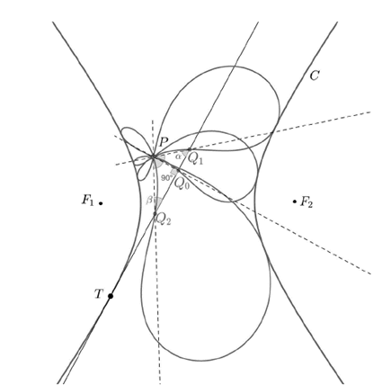
As shown in Fig. 3, the result of generalizing the pedal concept to any angle is a family of curves of the same nature. In most cases, the curves are tangent to curve C, although not always for smaller angles, as will be explained in further sections. The relationship between the traditional pedal curve (the one that is formed by the foot Q
0
of the line perpendicular to the tangent) and the rest of the curves of the family is a rotation with center P and angle ±(90o-α) and a homothety with center P and a factor of homothety

3. Limaçon as generalization of the pedal method
Using the traditional pedal concept for 90º, let C be the circle with polar equation r=a cosθ and P be the pedal point. The pedal curve obtained is the curve with the equation r=b+a cos θ [9,10]. This curve is a limaçon of Pascal.
Depending on the relative position of the pole P with respect to the center of the circle O and the radius r of the circle, it is possible to obtain a different type of limaçon [1], as shown in Fig. 4. If distance
 , the limaçon will be hyperbolic, and the double point of that limaçon will coincide with pole P
1
. If distance, which means that the pole is a point on the circumference, the limaçon will be a cardioid, that is, a parabolic limaçon. If distance
, the limaçon will be hyperbolic, and the double point of that limaçon will coincide with pole P
1
. If distance, which means that the pole is a point on the circumference, the limaçon will be a cardioid, that is, a parabolic limaçon. If distance
 , we obtain an elliptical limaçon.

Source: The authors.
Figure 4 Limaçons generated by the pedal method, for three different positions of the pedal point.
Consequently, other cases appear. If
 . the limaçon will be a double circle; if
 , the limaçon will be a trisectrix; and if
  , the limaçon will be a circle. Table 2 presents a classification of the limaçon according to
 for clarity.
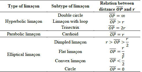
Standard classification distinguishes two types of elliptical limaçons. If the distance
 is between r and
 , that is,
  , then we obtain a dimpled limaçon. If the distance
 , the limaçon is convex, whereas if it is equal, the limaçon is flat.
As demonstrated in Section 2, changing the angle of the pedal does not affect the type of curve; however, it will affect the rotation and scale, as shown in Fig. 5.

4. Limaçon as a locus
The locus definition indicates that the limaçon of Pascal is the locus of points from which tangent t 1 to circle C 1 and tangent t 2 to circle C 2 form a constant angle, as shown in Fig. 6. Williamson, in 1899, defined it as the locus of the vertex of an angle of given magnitude, whose sides touch two given circles [5]. This locus generation method is then, not new, but certainly not well known; a review of recent literature showed that information on this generation method was scattered and incomplete [7,11].

However, the relationship between locus generation and pedal definition is less known or even completely unknown. The latter is a limit case of the locus definition of the limaçon that occurs when the radius of one of the circles becomes zero. This circle degenerates at a point that is the pedal point. Therefore, we can ensure the generalization of the pedal definition because the locus definition is valid for any angle, not only for perpendicularity.
To find the locus mentioned in the definition, let us consider the construction of such a locus. We begin by applying the inscribed angle theorem to find the locus of the points from which segment
 is seen under a given angle. This locus apparently does not have a name in English, so we will use the French term arc capable or Spanish term arco capaz. By tracing the tangents parallel to the lines that connect each point of the locus, we obtain four points, K, K',L, and L', as shown in Fig. 7, which, in pairs, describe the locus in question.

Therefore, given the data of two circles and an angle, we obtain four limaçons: the two shown in Fig. 8 and the two symmetrical with respect to the line between the centers of the circles to those ones. One of the two limaçons shown in Fig. 8 is generated by the two points K and K', where the interior tangent of one of the circles meets the exterior tangent of the other circle. The other limaçon is generated by points L and L', where the two exterior tangents or the two interior tangents intersect.
The limaçon, defined as a locus, might be seen as the definition of an isoptic curve of a pair of circles. The definition of an isoptic curve is the locus of points where a curve, or two in this case, is seen under a given fixed angle [12,13]. Extending this definition to the locus definition of the limaçon requires two leaps in reasoning: first, considering both circles as a single figure, and second, ignoring this consideration when the tangent to one circle goes over the other circle.

5. Additional properties
The locus and pedal generalization definitions allow us to deduce two additional properties of the limaçon.
5.1 Circle of similitude
In 1945, Butchart [6] reported a property derived from the locus definition. He realized that the double point or pole of the limaçon, which coincides with the pedal point in the pedal definition, is in the circle of similitude of the two circumferences. The diameter of this circle is the segment between the two centers of homothety of the two base circles, traced as shown in Fig. 9a. It is also defined as the locus of points viewing the two circles under equal angles and the locus of centers of homothety plus rotation that relate both circles. These three circles have the same radical axis [14], and therefore belong to the same pencil.
Because of the definition of the circle of similitude as a locus of points viewing the two circles under equal angles, the pole of the limaçon will be the only point of the limaçon that fulfills this property in addition to the property of the points of the limaçon as an isoptic curve of two circles [12, 13, 15], as shown in Fig. 9b.

Source: The authors.
Figure 9 (a) Circle of similitude in two circles belonging to an elliptical pencil or a hyperbolic pencil. (b) Pole of the limaçon as the point where the circle of similitude and the arc capable intersect.
Because the pole of the limaçon is in the circle of similitude, as well as in the arc capable of the locus definition, it is possible to find it as an intersection of both circles, as shown in Fig. 10. This provides a graphical construction to determine the pole of elliptic limaçons, defined as a locus.

5.2 Bitangent circles
Using the locus definition, any pair of circles with an angle provides four limaçons. The family of circles that generates the same limaçon has the same radical center; thus, they are all orthogonal to a circle c O , and that circle contains the pole of the limaçon.
We call the family of circles the bitangent circles of the limaçon, because for hyperbolic and parabolic limaçons, all the circles of the family are tangent at two points to the limaçon. For an elliptic limaçon, a portion of the family is bitangent, while the rest do not touch the limaçon at all (as the tangency point is imaginary).
The locus of the centers of all the circles of the family is another circle, c C , which is tangent to the pole of the limaçon to c O . The tangent points (T 1 and T 2 ) for each member c i of the family to the limaçon are those where c i intersects another circle, c j . The second circle, c j , is defined as passing through the center of c i and belonging to the orthogonal pencil of circles to the one formed by c C and c O, Examples of both hyperbolic and elliptic limaçons of this family of circles are shown in Fig. 11.

Source: The authors.
Figure 11 Example of bitangent circles with tangency points for hyperbolic (a) and elliptic (b) limaçons.
As can be observed in the figure, for hyperbolic limaçons, the pole is exterior to all c i of the family, and consequently there is always an intersection with c j . On an elliptic limaçon, the pole is interior; therefore, when c j , is small enough, it does not have a real intersection with c i , and the circle is not a tangent to the curve, which is not mentioned in [7], where this topic is treated as the solution to the problem proposed in [16]. Note that the pole of the limaçon belongs to this family as a degenerate case in which the radius is 0, which makes the pedal definition a particular case of the locus definition.
The family of bitangent circles has the following properties. Taking any two given circles from the family, it is possible to trace tangent lines from any point of the limaçon to those circles. The angle of two of those tangents (one for each circle) will be constant regardless of the point of the limaçon from which they are traced. Note that this is true only for one of the four possible combinations of tangents.
In addition, the angle between the two tangents to any of the circles of the family from the pole is always the same for any given limaçon, as shown in Fig. 12. For an elliptical limaçon, the tangents do not exist, whereas for a parabolic one, they form an angle of 180º.

Source: The authors.
Figure 12 Circles of the bi-tangent family viewed under the same angle from the pole of the limaçon.
There is an additional property in the singular case of a parabolic limaçon, that is, a cardioid. In a cardioid, the cusp is the same point as the pole, and all the bitangent circles are tangent to the curve at that point, as well as another. In addition, for any given two circles of the family, the angle between the tangents described above is the same as the angle between the two circles. This property is described in [6].
6. Conclusions
It is possible to generalize the pedal concept to any angle, generating a family of pedal curves that are related by rotation and homothety in which the pedal point is the center of both transformations, and the angle and factor of homothety are ±(90º-α) and k=1/sin α, respectively. In this manner, we can relate all the curves of the same family.
This definition is also applicable to the limaçon of Pascal because of its nature as a pedal curve. Thus, we can conclude, throughout its study as a locus, that the pedal definition of this curve is a limit case of the generalized pedal definition, which is also a limit case of the locus definition. This locus definition is not sufficiently described in the literature and neither are its implications; when observed through the perspective of the angular generalization of the pedal curve, it allows us to deduce some additional properties such as the relation between the circle of similitude, the arc capable, both being locus with angularity conditions, and the definition of the limaçon as an isoptic curve. In addition, it is possible to obtain a family of circles that are bitangent to the limaçon with interesting properties.
These properties are not only relevant to metric geometry but can also provide applications in the design and engineering fields owing to the extrapolation of the orthogonal property to general angularity, which allows greater flexibility in its applications. In addition, this research might lead to the generalization of other methods for generating pedal curves, with the possibility of obtaining and classifying the properties of these curves, which might have important implications in the field of metric geometry.

