


 Inglés (pdf)
 Articulo en XML
 Referencias del artículo
 Enviar articulo por email
 Citado por SciELO
  Citado por Google
  Similares en
SciELO
Similares en
SciELO  Similares en Google
 Permalink
1. Introduction
The evolution of the traditional (unidirectional) electricity system towards another peripheral is aimed at reducing the environmental impact, caused by the consumption of fossil fuels, and to improve of the efficiency of the network, minimising losses in the transmission and distribution of electricity to consumers. A relevant factor for this transition is the distributed generation units (DG) that take advantage of local energy resources, mainly renewable (sun and wind), helping meet the growing demand for energy. From the DG, the paradigm of a microgrid that aims to manage various types of generation, storage and loads to obtain high reliability emerges. They normally operate connected to the conventional network, but have the capacity to be self-sufficient [1].
One of the biggest challenges for DG and microgrids is finding mechanisms that determine the ideal capacity of generators and backup systems. In this sense,[2] finds the appropriate magnitudes, among others, of a wind generator and hydrogen storage. On the other hand,[3] details different techniques, divided into intuitive analysis, numerical methods and artificial intelligence, to improve the sizing of photovoltaic and wind systems. In addition,[4] proposes with linear programming, the adequate power of a mixed wind-photovoltaic generation system, as well as the savings that could be achieved in billing. However, the experiment design tool, especially the response surface methodology (RSM), has been little used to optimize the sizing of energy systems.[5] proposes this technique in an autonomous system composed of the photovoltaic-wind binomial and with battery backup. Likewise,[6] uses the method of factorial experimental designs to optimize the parameters of a monocrystalline photovoltaic panel.
This paper proposes the application of central composition design (CCD) -a branch of RSM- and regression to find optimal regions of expansion of photovoltaic arrays (AFV) and modification of the power supply of the turbine backrest system-generator, in the months of greater electric demand, to minimize the purchase of electrical power from the external supplier of the Center for Development of Renewable Energies (CEDER).
To achieve the objective, replicas generated by the simulator [7] were obtained, modifying the capacities of the seven AFVs and the power geometry of the turbine-generator backup system. At the same time, the best minimum values of purchased power (primary response) are identified by looking for the lowest values of the secondary response (standard deviation of the power supplied by the external network) according to the application "lower is better" of the Taguchi noise signal[8]; that is, the dual response technique was applied, simultaneously optimizing the mean and variance (represented by the standard deviation). The statistical analyses were developed with the statistical application software JMP (version 8.0.2). This paper is an extension of a work presented at the III Ibero-American Congress of Smart Cities (ICSC-CITIES 2020) and is structured as follows: section two describes the components and characteristics of the case study; then the methodology is presented where the statistical analyzes that give certainty to the use of the simulator to obtain the data are shown, showing a high degree of approach to the operational reality; the analysis factors, the number of replicates and, in general, the description of the two proposed techniques continue with the third section; the following section, with the help of the JMP, presents the results of the months under study; and, finally, the most relevant conclusions are pointed out.
2. Case study
CEDER is characterized by having several components manageable in the structure of its microgrid. Of the set of elements distributed here are studied photovoltaic generation (PV) and mini-hydraulics; Figure 1 shows these components[9]. About PV, there are 7 AFVs using different technology, five of monocrystalline silicon, one of polycrystalline silicon, and one of cadmium telluride. The nominal capacities of the AFVs are as follows: FV1037 = 5 kW, FV1038 = FV1044 = 4.5 kW, FV2000 = 12 kW, FV2005 = 12.5 kW, FV2010 = 16 kW and FV4360 = 23.5 kW, in total an installed power of 78 kWp. Moreover, the hydraulic plant is made up of a double-injector horizontal Pelton turbine, directly coupled to a three-phase asynchronous generator with a maximum power of 40 kW, delivering 400 V three-phase at a frequency of 50 Hz. For its operation, it takes advantage of a jump of 65 m and has two storage tanks with an approximate volume of 1637 m3 in the upper tank, and 2206 m3 in the lower; the distance between the two is 700 m. The supply pipe is made of PVC of 225 mm of internal diameter and consists of two sections of different walls, the first of 4 mm and the bottom of 6 mm, with the aim of withstanding the blows of the battering ram. The turbine operation is set to two power signal conditions, 45 and 60, respectively.

3. Materials and methods
3.1 Reliability of simulator responses
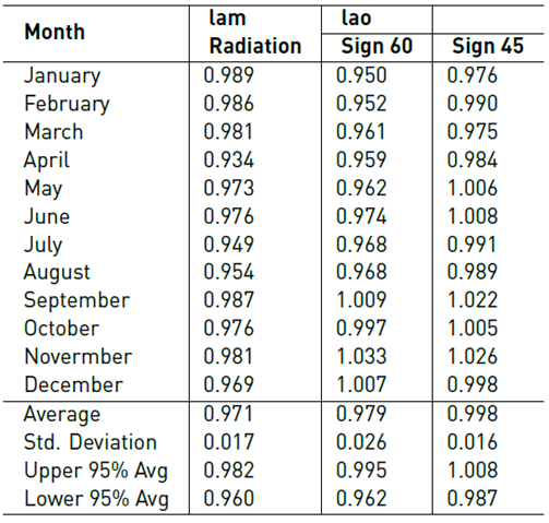
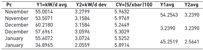
The experimental data are obtained with the aforementioned simulator; in order to demonstrate its reliability, two types of indexes were developed: approach to the measurement of solar radiation (Iam) and approach to the operation of the turbine-generator binomial (Iao), both represent the proximity of the information measured and that generated by the program. The simulator is considered reliable if the differences with the measured reality do not exceed 5% [10]. Iao was developed for the two possible input signal values. These indices were generated monthly, and 95% confidence intervals were obtained for all three. In addition, hypothesis tests were developed at 5% significance; the values tested in the hypotheses were 0.98 for the Iam and Iao signal 60, and 0.99 for the Iao signal 45; in all three analyzes, the value 1 represents the exact match to the measurements. Table 1 shows the monthly values of the indices. In the table, the 95% confidence intervals are very close to 1, and the averages obtained do not exceed 3% differences.
In this way, the simulator operates every 30 minutes for 17 intervals in the working hours of CEDER staff. It reports what is purchased or delivered in power units (kW) each day because it makes the sum of the differences between what is consumed and what is generated. The main reason for carrying out the monthly analysis is the billing; in this way, what is consumed, what is produced, and what is purchased from the external network are compared. Furthermore, in the best months of radiation, it is prioritized, from the simulator, not to deliver power to the supplier.
3.2 Dual response statistical models in RSM applying CCD and Regression.
The analyzed sample space is shaped as follows: two factors that are the increase of the nominal power capacity of the 7 AFVs (X 1) and the increase in the geometry of the turbine-generator backup system (X 2); two experimental responses, the monthly average daily purchased power (Y 1) and the standard deviation (SD) of . Y 1 (Y 2 ).By studying the simultaneous behavior of the two responses, the concept of dual response is formed.
MSR allows the researcher to inspect one or more responses that can be displayed as a surface when experiments look for the effect of varying quantitative factors on the possible values of a dependent variable or response; in other words, it tries to find the optimal values of the independent variables by maximizing, minimizing, or fulfilling certain response restrictions[11].
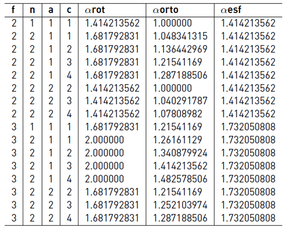
The most efficient experimental designs are those that allow the study of curvatures. The CCD design, originally called Box-Wilson [12], has been shown to require fewer trials to obtain reliable information. It is made up of an augmented full factorial design, with central and axial experimental points. The inclusion of central replicas favors the estimation of the general variance of the process of changes of values in the factors. Adding axial points, whose axial distance “a” can be defined by the researcher, gives qualities to the general variance profile, namely: (1) axial distance in phase with α = 1 generates a variance profile similar to the full factorial design with an additional level of study; (2) rotatable axial distance with value α > 1 creates a variance profile that tends to be constant as a function of the radius in the plane of a pair of studied factors; (3) orthogonal axial distance with value α ≥ 1 produces a variance profile that tends to be uncorrelated with the quadratic effects under study; (4) spherical axial distance with α > 1 value generates a variance profile that tends to be constant as a function of the radius in a triple of studied factors. Obviously, the number of replicas considered by the researcher will modify the values of these distances, except for the axial distance in phase, which is always α = 1 [11].
To exemplify the above, Table 2 shows some values of the factors under study (f), factorial replicas (n), axial replicas (a), central replicas (c). It can be seen in the table that the allowed values for the axial replicas must be less than or equal to the factorial replicas, the central replicas can be greater than or equal to the axial replicas and can exceed the replicas at each factorial point long as the statistical test of lack of fit (LOF) is not significant in all CCD design.
In the case study, the axial distance α = √2 was selected, with a rotatable feature to achieve the tendency that the SD is a function of the radius from the center to the limit of the sample space whose domain is the plane X1 − X2. The CCD used contains two factors, two replicates at each factorial point, two replicates at each axial point and four replicates at the central point, the reason for having selected this combination is to take care of a homogeneous weighting at all the noncentral points of the domain. On the other hand, increasing central replicates improves the estimation of SD, but increases the probability of making significant the LOF.
According to [14] the MSR using CCD formulates that this type of experimental design is based on approaches (1) and (2).
 be the response surfaces for the mean Y1 and standard deviation Y2 of the combined study process.


Where B and C are matrices of size k × k containing the second-order terms of the estimated coefficients of each response model; b and c are vectors of size k × 1 with the first order terms of the estimated coefficients of each model; b0 and c0 are scalar additive constants and x is a k × 1 vector of control or design variables. [15] details the general considerations for estimating models (1) and (2). On the other hand, the regression technique allows handling polynomials of any degree such that their effects are significant; this facilitates the study of curvature changes in fitted models. Regression uses least squares methods leaving the degree of the polynomial free. The theoretical support for this technique is based on the linear statistical model shown in Equation (3).

The previous model is expressed in a matrix in Equation (4):


The matrix X is of size nx(p + 1) where n ≥ p + 1, vector y is nx1, vector b is (p + 1)x1 and vector ε is nx1. Where n represents the total number of experimental points, p represents the number of parameters β j of the regressor variables xi1, xi2, . . . , xip, β0 represents an additive constant that, since there are no effects caused by the regressor variables, usually represents the mean of the response variable y. The estimator of vector b in expression (4) where X′ X is the variance-covariance matrix is defined, according to [16] by Equation (6).

For the regression analysis, as in the CCD technique, the same responses were studied (Y1, Y2), in this case they are represented by Equations (7) and (8).


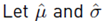
On the other hand, the increases allowed in the AFVs and the power of the backup system, as well as the values studied are found in Table 3.

The encoding of x1 and x2 shown in the table, is in the function of adjusting the domain of the sample space; these values are used in MSR and in regression. In particular, for the regression, the domain point (x1, x2) = (−α,−α) corresponds to the set of values introduced to the simulator of the current situation of CEDER.
The array of values used for Y1 and Y2 are found in Figure 2. The factorial points of the CCD are inscribed in the circle allowing for curvature analysis in four directions, and the rotatable axial distance is at the ends of the X1 and X2 axes. On the other hand, the regression technique leaves the SD profile free according to its possible polynomial adjustment.

The sample space for CCD is formed exclusively within the circle; on the contrary, the regression technique includes the outer points (Pcurrent, PaA, Pmax and PAa). Where X1 and X2 are the factors under study given in percentage increments. On the other hand, the geometry of the experimental points is shown in Table 4.
The responses Y1, Y2 were obtained by creating the experimental simulation of 20 and 28 years of operation for CCD and regression, respectively. When obtaining the data for each year, the number of days of power delivery (kW) per month to the supplier's electricity grid was counted. The categorical analyzes direct both studies to the months where greater participation of the supplier is required. The minimization in the regressions was carried out with the Solver complement of the Excel, under the condition of the Nonlinear Generalized Reduced Gradient (GRG) and the statistical analyses were done with [17].
4. Results
The selection of the months to study is based on the number of times power is delivered to the supplier. This categorical value allows them to be identified by obtaining the average daily power purchase. The measurement of SD was also considered as it is part of the CEDER decision criterion to cover its variations. The analysis of the days of power delivery to the external network is summarized in Table 5. The table shows the current conditions (Pc) of CEDER. November, December, and January have the lowest average deliveries, which are 0, 0, and 2.5 times in each month, respectively. Likewise, it can be observed in the space of possible increases given to the simulator, that the month of November contains the highest SD value; this defines it as the most important for the analysis. In this sense, Table 6 presents the three months with the highest power consumption of the CEDER.
It can be seen that November consumption is intermediate; however, it is the month with the highest SD and the highest percentage in the coefficient of variation (CV), confirming it as the key month in the study.

4.1 CCD analysis
November has a significant behavior of the variable Y1 in the effects: X1, X2, X1 X2, and
 , on the other hand, the variable Y2 is significant in the effects X1, X2 and
. The adjusted model can be observed in the prediction profile section of Figure 3. It should be noted that all statistical analyses meet significant relationships with α ≤ 0.05.
, on the other hand, the variable Y2 is significant in the effects X1, X2 and
. The adjusted model can be observed in the prediction profile section of Figure 3. It should be noted that all statistical analyses meet significant relationships with α ≤ 0.05.
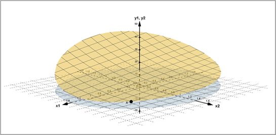
Figure 4 represents the three-dimensional behavior of Y1 (brown) and Y2 (blue). Point A (1,1) is the minimum obtained using the CCD technique and is valid for both responses.
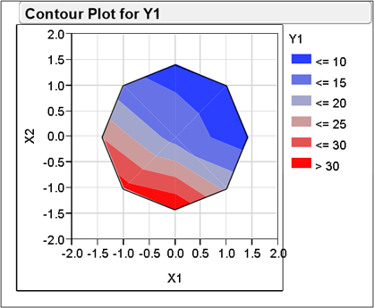
The contour plot, Figure 5, details the demand savings regions. The blue area represents the lowest demand section required. It is contained between the following points (x1, x2) : (−0.5, 1.2); (0, α); (1, 1); (α, 0); (1.3,−0.2); (0.7, 0); (0.5, 0.5); (0, 0.8) and (−0.5, 1.2) the most recommended area is the first quadrant of (x1, x2) ∈ E2.

In November, the region with the least required demand is intermediate in size, December covers a larger area, and January presents a smaller savings section. If greater savigns are needed, it is recommended to locate the increase decisions in the smallest region, so the effect in the months of December and November will be greater, and in January, an acceptable one will be reached, on average. Figure 6 splices the 3 previous zones. The most recommended area in all three cases is the proximity to point (1,1), that is, the first quadrant. Table 7 indicates the requested demand of the three months with the modification of X1 and X2 at that point.

If CEDER had the possibility of increasing the two factors to the point (1.1), the estimated average daily savings with reference to the current situation are: November (87.87%), December (83.53%), and January (74.04%). Additionally, a significant decrease in SD is achieved. On the other hand, the relative increase in CV is due to the greater decrease in Y1 compared to the decrease in Y2.
4.2 Regression analysis
Applying the regression technique for the month of November, the approximations of the two responses were obtained. Figure 7 shows their behaviors.

Unlike CCD, when doing regression, the cubic effect of X1 in both responses was significant, allowing to identify the change in curvature in this variable. Furthermore, it confirms that the FV contribution is dominant. By having a larger sample space, the minimum values of the responses are found at (alpha, 0.681) and (alpha, 0.969), respectively. For this reason, regression does not recommend increasing X 2 to alpha, since the value of both responses would be higher.
Since the primary response is more important than the secondary one, the results obtained in it are prioritized; in this way, regression suggests locating the minimum in (alpha, 0.68087). Figure 8 shows three-dimensional curvature changes of the cubic models of Y1 and Y2, as described in the prediction profile in Figure 7. The minimum point A (alpha, 0.681) is shown in Figure 8.
The boundary graph, Figure 9, details the demand-saving regions. The blue area represents the lowest demand section required. It is contained between the following points (−0.7, α); (α, α); (α,−0.25); (1.3,−0.25); (0.7, 0); (0.5, 0.5); (0, 0.8);(−0.6, 1.2) y (−0.7, α). Again the most recommended area is the first quadrant of (x1, x2) ∈ E2;this region contains what is proposed by the CCD technique.
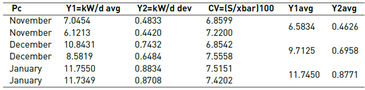

Figure 10 shows the regions where the best minimizations of the three months studied by the regression technique are achieved. The change in the order of the sizes of the areas lies in the fact of having increased the sample space allowing polynomial adjustments of a higher degree.
It can be seen that for the months of January and December, the regression favors the backup system, while for the month of November both techniques are more stable in their minimum region. Table 8 indicates the requested demand for the three months if X1 and X2 were modified at point A.

If CEDER had the possibility of increasing the two factors to point A, the estimated average daily savings with reference to the current situation are: November (92.77%), December (85.09%), and January (70.08%). In the comparative study of the three months, January is the month with the lowest savings and the highest SD.


5. Conclusions
The combined effects of the factors studied are non-linear as a whole. This is the reason for the use of dual response option response surface experimental designs. In both techniques, on average for the three months analyzed, at least 80% savings are assured in the region established by CCD for November.
The CCD technique weights the stability of the variance profile by standardizing the adjustment model to the second degree, while the estimated values have less variation compared to the simple regression technique; however, regression allows testing higher degree fits without controlling for variance. Therefore, it is recommended that CEDER decides to increase the power of the AFVs and the geometry of the turbine-generator backup, based on the region determined by CCD. In this sense, the increase in AFVs provides better results than the increase in storage geometry.

