Introduction

Gait, also referred to as bipedal locomotion, is a cyclic and fundamental movement that involves a sequence of repetitive events, initiating and concluding with the contact of the initial foot with the ground. This dynamic process encompasses a steady-state gait cycle, comprising the stance phase (when the reference foot is on the ground) and the swing phase (when the reference foot is off the ground). Gait constitutes a complex functional task that necessitates intricate coordination between numerous major joints within the human body, with particular emphasis on the lower limb ^1).

The modeling of human gait has garnered substantial attention from researchers in recent decades due to its profound implications in biomedical engineering. This interest arises from its applications in designing rehabilitation and assistive devices, as well as analyzing abnormal gait patterns and their consequences. Currently, the design of such devices, including exoskeletons, prostheses, and orthoses, often relies on empirical and trial-and-error approaches. Many of these devices are constructed and subsequently tested on individuals before obtaining valuable feedback, resulting in an inefficient and costly design process. Dynamic models provide a robust tool for designers by enabling the estimation of crucial kinematic and kinetic variables, such as angular displacements, velocities, accelerations, joint torques, and muscle forces. This facilitates optimal actuator selection and in-depth investigation into control techniques in order to achieve satisfactory performance before implementation ^(2-4). A rigorous and precise modeling approach enables the extrapolation of simulation results into practical applications, allowing designers to thoroughly evaluate their devices in a virtual environment before prototyping and human testing, thus reducing risks and costs ⁵. Additionally, dynamic modeling serves as a valuable resource for clinicians, rehabilitation experts, and researchers, enhancing their comprehension of both normal and pathological gait patterns and assisting in the identification of causes and effects related to abnormal movement patterns. A comprehensive understanding of the gait cycle, its parameters, and the principles underlying the musculoskeletal system and the central nervous system (CNS) provides essential insights for evaluating and treating locomotion dysfunctions in clinical environments ¹.

Research regarding the dynamic modelling of human gait can be categorized into two main fields: ¹ musculoskeletal models and ² biped robotics models. Musculoskeletal models ⁶ focus on the interaction and contributions of individual muscles, tendons, and ligaments during gait, emphasizing in the physiological aspects of bipedal locomotion. These models are highly intricate and computationally intensive, given their numerous degrees of freedom (DOF), diverting attention from the fundamental dynamics of the human gait. In contrast, biped robotics models aim at real-time gait control and the evaluation of kinematic and kinetic variables of joints and body segments. According to ⁷, biped robotics models can be divided into five groups: ¹ pendulum models, ² passive dynamic walkers, ³ zero-moment-point (ZMP) methods, ⁴ optimization-based methods, and ⁵ control-based methods.

Pendulum models are based on the principle of energy conservation, capturing the exchange between the kinetic and potential energy inherent in walking. Research in this area ranges from simple planar ^8,9 to 3D (10,11) and multi-mass pendulum models ^12,13. Pendulum models offer advantages in terms of simplicity, closed-form analytical solutions, and their ability to represent energy exchange principles during gait. However, they can oversimplify dynamics when certain joints and segments, such as the knee, ankle, lower leg, or foot, are not explicitly considered.

Passive dynamic walkers ^(14-16) are biped models that emulate a compass-like mechanism driven purely by gravity as they descend gentle slopes. These models do not involve any actuation or control of joint angles or torques at any point. During their descent, the leg follows a pendulum-like trajectory, and the swing foot’s contact with the ground is dictated by the conservation of angular momentum. Passive dynamic walkers are simple and efficient models suitable for investigating the fundamental principles of human gait, including the relationship between step length and velocity, energy expenditure, and the transition from walking to running. However, like pendulum-based models, they may oversimplify dynamics by neglecting certain joints and segments.

ZMP methods ^(17-19) focus on achieving bipedal walking by enforcing the body’s balance to follow predefined locations. Each ZMP represents a point on the ground where the net moment of active forces, including inertia, gravity, and external forces from actuators, is zero. The dynamic equations in this approach primarily serve to ensure balance constraints rather than coordinate the entire gait trajectory. ZMP methods are computationally efficient for the real-time control of biped robots. However, it is essential to note that preplanned ZMP locations do not precisely mimic human walking principles or the CNS’s control of gait.

Optimization-based methods ^{(7, 20, 21)} are computational approaches that seek to uncover the criteria governing human gait generation by the CNS. In these methods, the objective function - intended for optimization - typically represents a gait-related performance measure, such as dynamic effort, mechanical energy, metabolic energy, jerk, or stability. Constraints encompass the joint range of motion (ROM) and maximum joint torques. These methods offer insights into the relationship between gait and performance measures, shedding light on the working principles of human walking. However, they demand significant computational resources, are not well-suited for real-time applications, and rely on experimental data.

Control-based methods are deployed in humanoid robots to facilitate bipedal walking, allowing for interaction with the environment, responses to external disturbances, and real- time task execution. This approach closely approximates the natural control mechanisms of the human CNS, ensuring accurate analysis, estimation, and tracking of normal and pathological gait motions. Control-based methods can be classified into three categories: ¹ tracking control, ² optimal control, and ³ predictive control. Tracking control ^22,23 involves calculating input forces or torques required to achieve desired walking trajectories for body segments using kinematic feedback. In optimal control approaches ^{(24, 25)}, input forces or torques are treated as unknown variables in motion equations and are continuously optimized for the subsequent time step, also employing kinematic feedback. Predictive control methods ^{(5, 22)} are rooted in iterative finite horizon optimization, where online calculations are used to determine input forces or torques. This process minimizes a cost function incorporating kinematic feedback.

This paper introduces a dynamic model of human lower limb motion in the sagittal plane during the gait cycle. This model falls under the category of biped robotics and represents a hybrid approach incorporating elements of both pendulum and control-based methods. The model comprises two primary components: ¹ the plant model, founded on a multi-mass pendulum, and ² a closed-loop PID controller. The plant model captures the forward dynamics of human gait, employing the Euler-Lagrange formulation while considering the lower limb as consisting of three segments (thigh, lower leg, and foot) and three joints (hip, knee, and ankle). The PID controller is integrated to estimate the joint torques necessary for replicating human gait reference trajectories. It constitutes a potent tool for the design of rehabilitation and assistive devices, facilitating joint torque estimation, kinematic variable analysis, optimal actuator selection, and the exploration of control techniques.

Dynamic model

As mentioned in the introduction, the dynamic model proposed for human lower limb motion encompasses two essential components: ¹ the plant model and ² a closed-loop PID controller. The plant model (the core of the dynamic model) represents the forward dynamics of human gait, and the closed loop controller simulates the working principle of the neuromusculoskeletal system and the CNS.

It is worth noting that the scope of this dynamic model is specifically confined to the sagittal plane. This deliberate limitation stems from the recognition that the motion and dynamic effects of the lower limb within the frontal and transverse planes exhibit diminished relevance compared to those within the sagittal plane ¹.

Plant model

The plant model, responsible for capturing the dynamics of human lower limb motion, is meticulously formulated using the Euler-Lagrange formulation. This mathematical framework is applied to the system depicted in Fig. 1, which comprises three lower limb segments (thigh, lower leg, and foot) interconnected by three joints (hip, knee, and ankle). Each of the lower limb segments is modeled as a rigid bar by specific attributes. These attributes include length L _n , mass m _n , and the proximal gravity center l _n . These segments are positioned at angular positions θ _n relative to the vertical axis. To distinguish between the individual segments within the model, subscripts are employed as follows: ‘1’ for the thigh, ‘2’ for the lower leg, and ‘3’ for the foot. The foundation of this modeling

Figure 1 Representation of human lower limb for dynamic modeling 

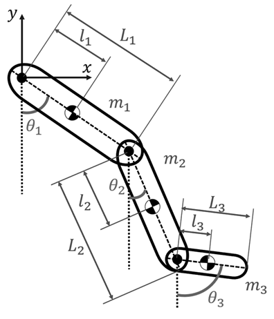
framework is established in a fixed coordinate system with its origin situated at the hip joint.

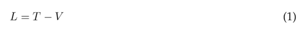
The Lagrangian L is established as the difference between the system’s kinetic energy T and its potential energy V:

The kinetic energy is defined by Eq. (2), which incorporates the kinetic energy of each individual segment. In this equation, v _n represents the linear velocity, J _n denotes the moment of inertia, and θ˙n represents the angular velocity.

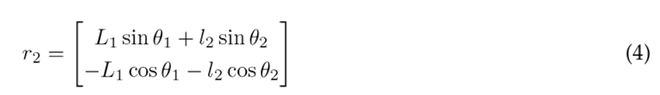
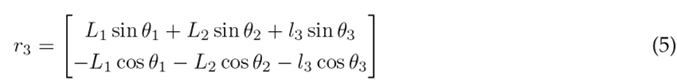
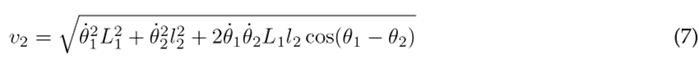
The linear velocity can be expressed as the magnitude of the first derivate of the position vector r _n of the gravity center for each segment: v _n = |r˙ _n |. The centers of gravity for the thigh, lower leg, and foot are situated at positions r ₁, r ₂ and r ₃, respectively:

Therefore, the linear velocities of the thigh, lower leg, and foot are established as:

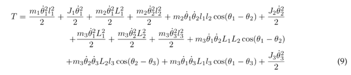
Substituting Eqs. (6), (7), and (8) into (2) results in the following expression for the kinetic energy of the system:

The potential energy is defined by Eq. (10), which incorporates the potential energy of each individual segment. In this equation, g denotes the gravity, and h _n represents the height of the center of gravity relative to the coordinate system.

The height of the center of gravity for the thigh, lower leg, and foot can be expressed in terms of the angular displacement as:

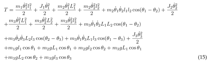
Substituting Eqs. (11), (12), and (13) into (10) results in the following expression for the potential energy of the system:

Eqs. (9) and (14) are substituted into (1) to obtain the Lagrangian of the system:

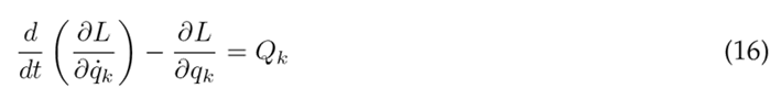
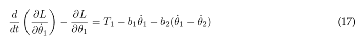
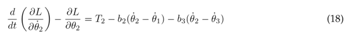
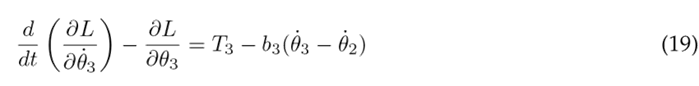
The Euler-Lagrange formulation is established by Eq. (16), where k represents the DOF, q _k the set of generalized coordinates, and Q _k the set of external (non-conservative) forces applied to the system. In the context of the system under consideration, there are three DOF associated with the three joints of the lower limb. The external forces encompass the torque T _n acting at each joint and the viscous damping, with b _n representing the viscous damping coefficient. The Euler-Lagrange formulation is applied as seen in Eqs. (17), (18), and (19) for the hip, knee, and ankle, respectively.

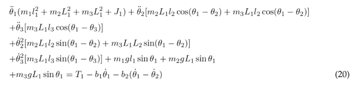
The equations above are solved resulting in the nonlinear second-order differential Eqs. (20), (21), and (22), which describe the motion of the thigh, lower leg, and foot, respectively.

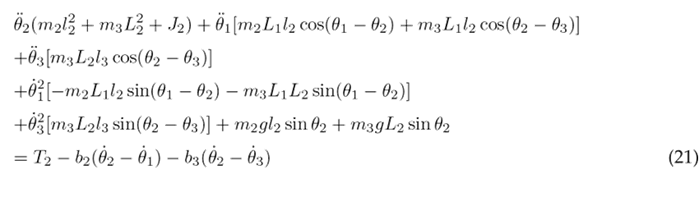
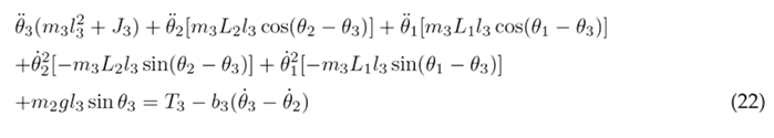
To simplify the aforementioned differential equations, certain parameters are combined into the following constants: following constants: c ₁ = m ₁ l ₂ + m ₂ L ² + m ₃ L ² + J ₁ , c ₂ = m ₂ L ₁ l ₂ , c ₃ = m ₃ L ₁ L ₂ , c ₄ = m ₃ L ₁ l ₃ , c ₅ = m ₁ gl ₁ , c ₆ = m ₂ gL ₁ , c ₇ = m ₃ gL ₁ , c ₈ = m ₂ l ² + m ₃ L ² + J ₂ , c ₉ = m ₃ L ₂ l ₃ , c ₁₀ = m ₂ gl ₂ , c ₁₁ = m ₃ gL ₂ , c ₁₂ = m ₃ l ² + J ₃ , and c ₁₃ = m ₃ gl ₃ . As a result of these simplifications, Eqs. (23), (24), and (25) are obtained.

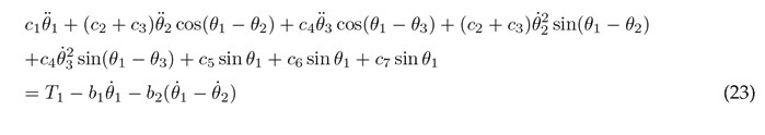
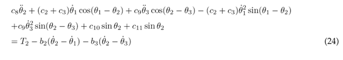
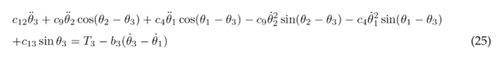
Eqs. (23), (24), and (25) are solved for the highest order derivatives θ¨1, θ¨1, and θ¨3 respectively, in order to obtain the following set of motion equations:

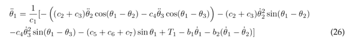
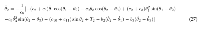
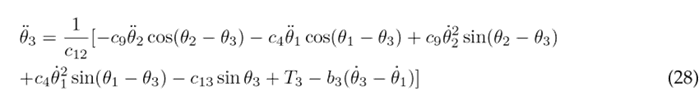
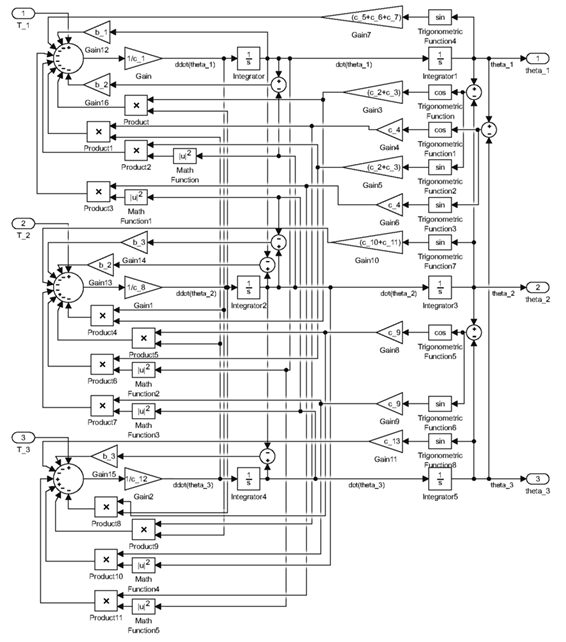
This plant model of human lower limb motion in the sagittal plane was implemented in MATLAB’s Simulink, and it utilizes the non-linear second-order differential Eqs. (26), (27), and (28), as illustrated in the block diagram presented in Fig. 2 . The inputs to this model consist of the joint torques (T ₁, T ₂ and T ₃) measured in units of (N m), while the outputs are the angular displacements of the thigh, lower leg, and foot (θ ₁ , θ ₂ and θ ₃), reported in units of (rad).

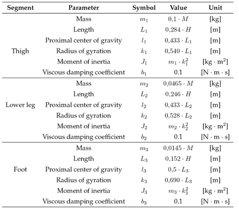
The parameters that make up the plant model are detailed in Table I. These parameters are derived trough an anthropometric analysis that relies on two primary factors: the body mass M and the height H of the individual. The mass of each segment and its corresponding length are linked to the individual’s body mass and height, and the gravity center and radius of gyration are associated with the segment length (26, 27).

Table I Parameters of the plant model for human lower limb motion 

Closed-loop controller

The neuromusculoskeletal system was conceptualized within a closed-loop feedback control scheme. In this structured framework, the body’s segments and joints comprise the plant, muscles serve as the actuators, and an array of sensors, including proprioceptive and tactile sensors alongside visual and vestibular systems, act as sensory inputs. Overseeing this complex system is the CNS, functioning as the controller ²⁸. The CNS receives input signals representing desired positions or reference trajectories, generated by the brain. These inputs are compared against real-time segment locations to compute tracking errors, which, in turn, guide the CNS in sending neural signals to muscles. These signals prompt the exertion of forces on the skeletal system, thereby producing joint torques to achieve the desired motion.

To simulate the neuromusculoskeletal system and the CNS, the model employs three angular displacement feedback PID controllers for the hip, knee, and ankle. Fig. 3 illustrates these controllers.

Their inputs are tracking errors, computed as the difference between reference trajectories and actual segment angular displacements. The controllers’ outputs represent the joint torques required for carrying out the intended motion. These PID controller outputs feed directly into the plant model, depicted in Fig. Fig. 2. For the sake of clarity and comprehensibility, this plant model is encapsulated within a Simulink subsystem block, as illustrated in Fig. 3 .

Figure 2 Plant model of human lower limb motion in Simulink 

Figure 3 Closed-loop PID controllers implemented in the plant model in Simulink 

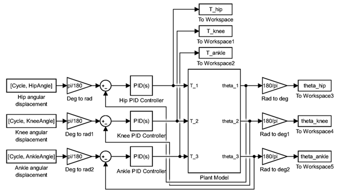
A notable aspect of this modeling process pertains to unit conversions. While the plant model operates with angular displacements measured in radians, reference trajectories are presented in degrees. To ensure consistency, unit conversion is performed using specialized gain blocks designated as Deg to rad and Rad to deg. These blocks facilitate the transformation of reference trajectories from degrees to radians before tracking error computation. Furthermore, the angular displacements of the dynamic model are converted from radians to degrees for visualization purposes.

PID control is a classical closed-loop control technique defined by the Laplace domain transfer function shown in Eq. (29). It comprises three essential constants: proportional K _p , integral K _i , and derivative K _d . These constants play distinct roles in shaping system behavior: the proportional constant enhances the system’s responsiveness; the integral constant reduces steady-state error; improving precise tracking of reference trajectories; and the derivative constant manages the tracking error’s evolution over time ².

To optimize controller performance, an experimental tuning process was conducted on the plant model. The objective was to achieve optimal tracking performance while ensuring that joint torques remained within the reported maximum values for normal gait ²⁹. The tuning process resulted in PD controllers for the three joints, configured as follows: the hip controller was configured with K _p = 10,000 and K _d = 1, the knee controller with K _p = 1,000 and K _d = 10, and the ankle controller with K _p = 1,000 and K _d =10

Simulations and results

Simulations of the dynamic model were conducted using human gait reference trajectories obtained from ²⁹, with due consideration to the anthropometric data (body mass and height) reported in their research. These reference trajectories comprise the angular displacement of the hip, knee, and ankle joints during the gait cycle of healthy male adults.

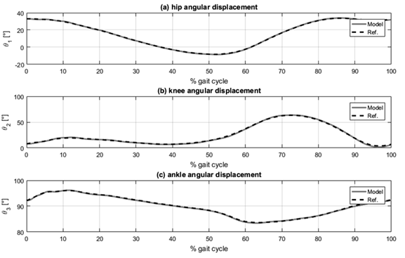
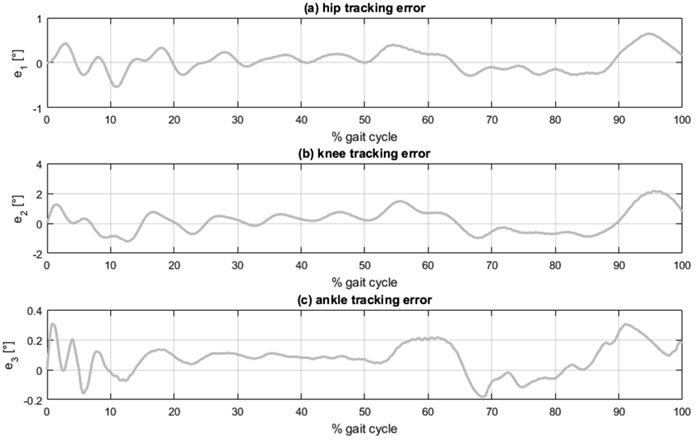
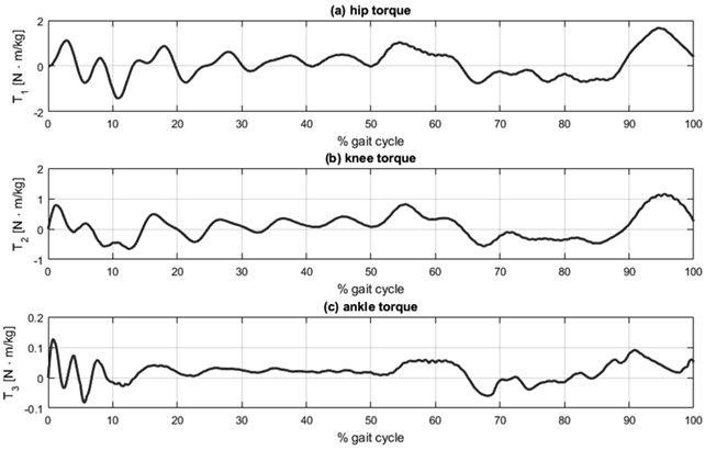
Graphical simulation results are presented in Fig. 4, Fig. 5 and Fig. 6, each consisting of three plots corresponding to the three lower limb joints: (a) hip, (b) knee, and (c) ankle. Fig. 4 shows the tracking of angular displacement, with the reference trajectory represented as the dotted line and the angular displacement of the segment in the dynamic model shown as the solid line. Fig. 5 illustrates the tracking error regarding angular displacement, calculated as the difference between the reference trajectory and the angular displacement of the segment. Fig. 6 presents the normalized joint torque during the execution of the desired gait reference trajectory. This normalization is established relative to the individual’s body mass.

Figure 4 Angular displacement tracking: (a) hip, (b) knee, and (c) ankle 

Figure 5 Angular displacement tracking error: (a) hip, (b) knee, and (c) ankle 

Figure 6 Joint torque: (a) hip, (b) knee, and (c) ankle 

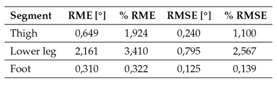
The assessment of angular displacement tracking in the dynamic model involved the application of two key metrics: the relative maximum error (RME) and the root mean square error (RMSE), both in magnitude and as a percentage. These metrics were calculated using Eqs. (30) to (33), where θ _d represents the reference trajectory, θ _n model, and N denotes the signal length ². Quantitative results from this evaluation are presented in Table II, encompassing data for the three segments under consideration.

Table II Angular displacement tracking errors of the dynamic model 

The analysis of the graphical results, as depicted in Figs. 4and 5, reveals that the most significant tracking errors tend to appear during the peaks of the reference trajectories. While PID controllers can be finetuned to minimize tracking errors, it is essential to recognize that pushing these controllers to achieve such minimal errors could result in joint torques surpassing the reported values for normal human gait ²⁹.

Angular displacement tracking was effectively accomplished with errors remaining under 2.2 (°) in magnitude and within a margin of 3,5 % for all three segments considered. Notably, the lower leg segment exhibited the most substantial tracking errors. This can be attributed to the dynamic interactions between the thigh and foot segments, which, in turn, impact the lower leg’s overall performance. Despite these challenges, the tracking errors for the thigh and foot segments were effectively constrained below 0,65 (°) and 2 %.

Conclusions

This paper presented the development of a dynamic model for human lower limb motion in the sagittal plane during the gait cycle. The dynamic model was composed of two primary components: (1) the plant model and (2) a closed-loop PID controller. The plant model served as the foundation for understanding the forward dynamics of human gait. It was constructed based on a multi-mass pendulum, encompassing three lower limb segments (thigh, lower leg, and foot) and three joints (hip, knee, and ankle). The governing nonlinear second-order differential equations of the plant model were derived trough Euler-Lagrange formulation and subsequently implemented in MATLAB’s Simulink. To replicate human gait reference trajectories and simulate the functioning of the neuromusculoskeletal system and the CNS, a closed-loop PID controller was integrated to the plant model for tracking angular displacement.

Simulations were conducted using human gait reference trajectories sourced from healthy adult males. The accuracy of angular displacement tracking was rigorously assessed, quantified by two key metrics: the relative maximum error (RME) and the root mean square error (RMSE). The simulation results affirm the reliability of the dynamic model, demonstrating its ability to faithfully reproduce human gait trajectories with a high degree of precision. The errors observed were consistently below 2,2 (°) in magnitude and 3,5 % for all three considered segments (thigh, lower leg, and foot).

Within the domain of dynamic human gait modeling, this model resides within the realm of biped robotics, offering a unique hybrid approach that amalgamates pendulum and control- based methodologies. This model stands as a potent tool, empowering the design of rehabilitation and assistive devices, such as exoskeletons, prostheses, and orthoses. It enables crucial functionalities, including joint torque estimation, analysis of kinematic variables, optimal actuator selection, and exploration of advanced control techniques