


 Inglés (pdf)
 Articulo en XML
 Referencias del artículo
 Enviar articulo por email
 Citado por SciELO
  Citado por Google
  Similares en
SciELO
Similares en
SciELO  Similares en Google
 Permalink
INTRODUCTION
Globally, around 21.7 million tons of peas are produced on more than 2.78 million hectares. Countries such as China and India cover 75.5% of production (FAO, 2019). In Colombia, peas are the second most important legume, after bean cultivation. Fenalce (2010) noted that production requires a significant amount of labor, generating around 15 thousand direct jobs. It is produced with greater intensity at high altitudes >2,000 m a.s.l., so departments such as Nariño, Cundinamarca, Boyaca and Tolima cover more than 90% of the domestic production (Agronet, 2018).
The main biotic factors that limit production are described below. Ascochyta spp. reduces pea yield by 10-60% through deterioration of the pod and grain, decreasing commercial value (Bretag et al., 2006). In the initial stages, pests affect crop establishment by up to 100% (Ciancio, and Mukerji, 2007). Peas are recognized as a low-competition plant that requires strict weed control (Díaz and Zapata, 1990; Zamorano et al., 2008). It also serves as a host for pests and diseases (ICA, 2012). Finally, weeds have the greatest impact on crop losses (DANE, 2015).
Weed identification and quantification is required to know weed biodiversity, to know the effect of weeds in crop yield or to know the effect of the control strategies on weeds and different objectives require different sampling strategies and several variables measured, such as density, which measures the number of individuals for a given area and coverage which is the percentage of area covered by weeds on the ground (Blanco and Leiva, 2010; Jamaica and Plaza, 2014).
Weed evaluation using conventional sampling methods are time consuming, so, methodologies or tools that improve these techniques in terms of efficiency and precision are needed. Several authors have observed that these conventional methods are subjective and unreliable (Andújar et al., 2010; González-Andújar et al., 2011; Nkoa et al., 2015; Zimdahl, 2018). Within the framework of the fourth industrial revolution, the use of sensors and image processing can improve weed infestation assessments.
Remote sensing aims to recognize terrestrial surface characteristics, which are recorded by a sensor (Sobrino, 2000). Spectral and morphometric properties allow to detect weed populations and differentiate them from the soil and crop (Jurado-Expósito et al., 2003). The main characteristics of sensors are spectral, spatial and temporal resolution. Spectral resolution is the number of bands (nm) that sensors can get separately. Spatial resolution is the physical area that each pixel represents in the image. This area depends on the height at which the image is taken and its resolution. Finally, temporal resolution refers to the how often data of the same area is collected by sensors (Castillejo-González et al., 2014; Torres-Sánchez et al., 2015).
For example, satellites systems have low temporal resolution because they provide information every time you fly over the area of interest and low spatial resolution since they are located kilometers above the surface. In contrast, R-PAS (Remote Pilot Aircraft System) overcomes these problems because it is more frequently available and is found at a low altitude, but it is still not suitable for weed evaluations in herbicide efficacy tests since it requires a very high spatial resolution (mm / pixel) and high temporal availability.
On the other hand, efficacy bioassays are essential for the evaluation process and are required for the registration of chemical pesticides for agricultural use (CPAU) in Colombia. In accordance with Decision 436 of the Andean Community of Nations (ACN), CPAU efficacy bioassays must be carried out, and the testing protocol must be presented so competent authorities can supervise the method for subsequent approval (CAN, 1998).
These efficacy bioassays are essentially the percentage of control over a pest organism under treatment as compared with an untreated area. In weeds, the most used evaluation method is visual estimation of the coverage, counts and dry mass, using squares of 0.25×0.25 m or 0.5×0.5 m as a sampling unit. This method must be supported by statistical analyses with sufficient repetitions, randomization and untreated areas (ANDI and ICA, 2015).
However, in Colombia, there is no record of registered pre-emergent herbicides in pea crops; however, there is a record for crops such as carrot, onion, and tomatoes, etc. (ICA, 2019). Pre-emergence herbicides are applied to the soil after planting and before crop emergence. This practice aims to mitigate the negative effect of the crop-weed competition in early crop stages (Wágner and Nádasy, 2006; Zamorano et al., 2008).
Pre-emergent herbicides were tested to control weeds in a pea crop. It was found that linuron and metribuzin, at doses of 3 kg and 0.75 L ha-1, had 98 and 100% effectiveness (Espinoza and Ormeño, 1989). The weeds were controlled at 90% during the first 45 days after sowing (DAS) with flumozazin and acetolachlor at a dose of 150 mL and 1 L ha-1, respectively. Lescano et al., (2017) obtained 90% control during the first 45 DAS, and a large portion of tests with mixtures showed control over 80% under field conditions in that region. A mixture with imidazolinones is recommended (Yanniccari et al., 2017). Successful control with pendimetalin at pc 1.5 kg ha-1 and fluchloralin at pc 1 kg ha-1 has been reported (Rana, 2002). An herbicide combination trial of pendimethalin at pc 1 kg ha-1 in pre-emergence had better weed control, but applications of imazetapir + imazamox 60 g ha-1 in post-emergence (45 dds) may be an alternative for mixed weed control (Mawalia et al., 2016).
In these trials, plants were randomly sampled. The data were evaluated in conventionally (severity scales, counts and coverage). Given the shortcomings of these methods, new ones are needed for assessing weed control effectiveness using emerging technologies framed in the fourth industrial revolution. Therefore, the objective was to evaluate different pre-emergent herbicides and doses in a pea crop and validate the use of multispectral images, since remote sensing of weed infestations can be more precise and may allow site specific weed management in order to reduce herbicide use by up to 70% (Weis and Sökefeld, 2010).
MATERIALS AND METHODS
Peas of the Vizcaya variety were sown in the greenhouses of the Faculty of Agricultural Sciences of the Universidad Nacional de Colombia, Bogota campus. The treatments were tested using a complete randomized design with two factors (herbicides and doses). The treatments consisted of an untreated area, five herbicides, and two doses level with three replications. The untreated treatment was replicated six times to obtain a balanced experimental plot. Thus, 36 experiment units (2.0×3.3 m) were established (Tab. 1).
Table 1. Herbicides and dose evaluated.
| Herbicide | Dose level | Registered crop use (c.p.) | Units | Dose (c.p.) | Dose (a.i.) |
|---|---|---|---|---|---|
| Linuron | DC | Carrot | g ha-1 | 1,500 | 900 |
| Linuron | MD | Carrot | g ha-1 | 750 | 450 |
| S-Metolachlor | DC | Beet | mL ha-1 | 750 | 698 |
| S-Metolachlor | MD | Beet | mL ha-1 | 375 | 360 |
| Metribuzine | DC | Potato | mL ha-1 | 1,000 | 576 |
| Metribuzine | MD | Potato | mL ha-1 | 500 | 288 |
| Oxifluorfen | DC | Onion | mL ha-1 | 1,100 | 633.6 |
| Oxifluorfen | MD | Onion | mL ha-1 | 550 | 316.8 |
| Pendimetalin | DC | Onion | mL ha-1 | 2,000 | 960 |
| Pendimetalin | MD | Onion | mL ha-1 | 1,000 | 480 |
DC: Commercial dose; MD: half of the commercial dose; c.p: commercial product. a.i: active ingredient.
Weed presence, in terms of soil cover percentage at 12, 24 and 36 DAS, was assessed with two methods: conventional human visual estimation and multispectral images. In the former, the data were obtained by a person who was an expert. In the latter, a Parrot Sequoia® multispectral sensor, mounted in a frame, took images at 1.6 m (Fig. 1). This height was chosen because a high spatial resolution was needed to evaluate the trial and only one image was needed for each experiment unit. The sensor used a camera with 16 Mpx RGB and spatial resolution of 0.22 cm2 per pixel at 2 m, with four monochromatic bands: red (660 nm), green (550 nm), near-red (735 nm) and near infrared (790 nm).

Figure 1. Small (0.6 m) support structure of the camera: (A) Top view of the frame, (B) front view of the frame and (C) sensor adapted to the frame. Adapted from Puerto (2018).
To process the images, software was developed using an algorithm known as fuzzy C-means. This version is a modified K-means that associates the probability of a pixel belonging to a certain class (Bai et al., 2017). The multispectral camera obtained false color images with the appearance of a simple RGB image; for example, a false green is shown in figure 2.

Figure 2. Multispectral image of the false green. The R, NIR and G bands were used as RGB representation components (Puerto, 2018).
The fuzzy C-means algorithm is supported in the following function (1):
where
The optimal values must be found (2):
The solution of this optimization problem yields the following result (3) (4):
The implementation of the algorithm is carried out as follows:
Randomly start the values
Find the centroid using Eq. (4).
Calculate new values of
Calculate the objective function of Eq. (1).
Repeat steps 2 to 4 until the algorithm converges.
The convergence of the algorithm depends on a minimal variation between iterations. Figure 3 shows the resulting image when figure 2 is processed.

The pea crop is denoted by the magenta pixels. Notably, the resulting image evidenced other types of objects that were less evident in the original image, especially on the ground (Puerto, 2018). Finally, the cluster of interest was transferred to the original image to demonstrate detection and subsequently find its coverage (Fig. 4).

The variable coverage was transformed into efficacy by calculating the Abbott’s corrected efficacy (Eq. 5), where 0 means that there was no control compared to the untreated plants, and 100 means there was control of all weeds.
where, Td is the infestation of the treated plot after applying the treatment, and Cd is the infestation of the untreated plot.
A harvest sampling was also carried out in the central line of each plot. In the field, crop establishment was determined by measuring the number of plants and number of pods, and, in the laboratory, yield variables such as number of grains per pod and weight of 50 g were measured to determine the yield per plot in t ha-1.
The yield was estimated with Eq. 6:
where, NPP is the number of plants per plot, PPP is the number of pods per plant, GPD is the number of grains per pod, PCG is the weight of 50 g, and AP is the area of the plot.
Finally, the statistical package R was used to determine statistical assumptions of normality. The analysis of variance ANOVA was applied to reveal significant differences for the pre-emergence herbicide treatments and doses. Agreement between the evaluation methods (human vs. machine) was analyzed with the Intraclass Correlation Coefficient (ICC) in the “irr” package (Gamer et al., 2010), as recommended by Andújar et al. (2010), and configured to a “one-way” model, “single” unit, and the Bland-Altman plot to determine agreement between both data sets.
RESULTS AND DISCUSSION
In the experimental plot, the floristic composition had 90% coverage by broadleaf species and 10% by narrow leaf species (grasses) (Tab. 2).
Table 2. Weed species found in the experimental plot.
| Group | Species |
|---|---|
| Broadleaves | Sonchus oleraceus L., Oxalis corniculata L., Stellaria media L., Capsella bursa-pastoris L., Trifolium repens L. |
| Grasses | Poa annua L. |
When comparing the two weed coverage estimation methods, the ICC was 0.967 with a p-value of 0, which showed excellent agreement between the methods, meaning that one could replace the other (Giavarina, 2015; Osorio et al., 2020). In the Bland-Altman plot, the X-axis represented the means of coverage, while the Y-axis represented the difference between the methods. Black lines represent the confidence limits of the methods (Fig. 5), which fall within the range of acceptable tolerance limits (-12 to +17), which is acceptable but depends on the use of the data and the sensitivity of the bias. The blue line was obtained with the values estimated with the regression model. The negative slope was interpreted as an overestimation of coverages of conventional human visual estimation versus the multispectral image procedure (Osorio et al., 2020), similar to the results of Benlloch et al. (1996) despite the older image processing methods.

The corresponding analysis for data recorded at 36 DAS (Tab. 3) compared the treatment means with the Tukey test (Fig. 6). The ANOVA showed differences between the treatments for weed control. There were no differences for the doses, and there was no significant interaction between the herbicides and doses. The Tukey test for the treatments indicated that oxifluorfen and metribuzin had the highest efficacy; that linuron did not have adequate control of the weeds, similar to the results of (Banga et al., 1998), and that metolachlor and pendimethalin (recommended for grass control) did not control the weeds. The latter was explained by a large presence of broader leaves in the treated plots. The data at 12 and 24 DAS are not shown because they did not differ from the data at 36 DAS.
Table 3. ANOVA for herbicide efficacy data recorded at 36 DAS.
| Df | Sum Sq | Mean Sq | F value | P(>F) | |
|---|---|---|---|---|---|
| Herbicide | 5 | 52793 | 10559 | 80.951 | 3.17·10-14 |
| Dose | 1 | 9 | 9 | 0.068 | 0.796 |
| Herbicide×Dose | 5 | 296 | 59 | 0.453 | 0.807 |
| Residuals | 24 | 3130 | 130 |
Df: degrees of freedom; sq: squares.
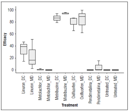
Figure 6. Herbicide efficacy at 36 DAS. Statistical differences between two groups: orange (good control) and green (poor control). DC: full commercial dose; MD: half of the commercial dose, see table 1.
Previously, the herbicides with the best efficacy were reported as metribuzine and oxifluorfen. However, as shown in figure 7, the crop establishment for oxifluorfen did not exceed 67%, with yield like that obtained with the herbicides linuron, metolachlor at medium dose, and pendimethalin. Tests carried out by Semidey and Almodóvar (1987) showed that, with a commercial dose of 0.6 L ha-1 of a.i., Cajanus cajan has phytotoxicity that disappears in 9 weeks, without altering yield.

Figure 7. Crop establishment (%) at 36 DAS. DC: full commercial dose; MD: half of the commercial dose, see table 1.
There was interaction between the treatment and dose for yield (Tab. 4) since the metribuzine doses had the biggest difference. At an a.i. dose of 0.6 L ha-1, 33% establishment was reached, with a yield of 0.13 t ha-1 (the lowest). The 0.3 L ha-1 dose reached 90% establishment, with a yield of 2.37 t ha-1 (the highest). At 36 DAS, a control efficacy of 88% of the weed cover was achieved, which was the optimal result and the treatment recommended by this assay (Fig. 8). This contrasting result may have been due to the loss of selectivity of the herbicide to the crop from the dose. Wágner and Nádasy (2006) tested this herbicide at higher doses, finding similar results.
Table 4 ANOVA for grain yield (t ha-1) by treatments, dose and interaction.
| Df | Sum Sq | Mean Sq | F value | P(>F) | |
|---|---|---|---|---|---|
| Herbicide | 5 | 4.62 | 0.924 | 4.311 | 0.00611 |
| Dose | 1 | 1.319 | 1.3189 | 6.153 | 0.02053 |
| Herbicide x Dose | 5 | 7.069 | 1.4138 | 6.597 | 0.00054 |
| Residuals | 24 | 5.143 | 0.2143 |
Df: degrees of freedom; sq: squares

Figure 8. Estimated yield for each treatment (t ha-1). DC: full commercial dose; MD: half of the commercial dose, see table 1.
CONCLUSION
The weed coverage assessment with sensor and image processing was validated and had contrasting advantages over the conventional visual-human method since it was faster and more precise. This methodology can be used to standardize coverage samples for herbicide efficacy tests, especially for register trials. Further studies could fully assess the economic advantages of using this technology.
The Metribuzine application at MD was the best treatment for controlling weeds, obtaining the highest crop establishment and grain yield. Further studies could find the adequate doses since MD (half of commercial dose) was enough to control the weeds.
Metolachlor and Pendimethalin were not effective at controlling the weeds because of the predominance of broad leaves in the pea crop. Oxyfluorfen had the highest efficacy for weed control but also had the greatest phytotoxic effect on the pea plants; therefore, it is not recommended as a pre-emergence treatment in pea cropping systems.
Linuron was ineffective for controlling the weeds probably because the tested doses were low.

