


 Inglés (pdf)
 Articulo en XML
 Referencias del artículo
 Enviar articulo por email
 Citado por SciELO
  Citado por Google
  Similares en
SciELO
Similares en
SciELO  Similares en Google
 Permalink
1. Introduction
Over recent decades, the increased levels of contaminants that can affect human health or damage air quality have caused governments to introduce legislation to regulate air pollution levels [1]. Structuring programs and regulations in order to achieve an efficient, timely, complete and practical surveillance of air quality and its harmful effects on the population is crucial [2]. In [3] the differences between E.U. and U.S. air protection policies and legislation are discussed. Air quality management is a complex problem that should be examined on different geopolitical levels using a set of instruments. The common objective of all these instruments must be, however, to ensure the best possible air quality [3].
Consequently, mathematical models have been used to determine the concentration of the pollutant in region Ω. These models are algorithms that can quantify the relation between concentration and emissions, allowing us to establish the consequences of past and future scenarios.
Depending on the methodology, dispersion models can be classified as being one of the following four types: 1) box models, 2) Lagrangian, 3) Gaussian models, and 4) Computational models of fluid dynamics. The first models are based on conservation of mass and they consider the region to be a box. The second type of models consider air part as a box with an initial concentration of contaminants moving in the direction of the wind. They also consider concentration to be a product of a source term and a probability density function when the contaminant moves from one point to another [4]. The third type, known as Gaussian models, assume that the contaminant plume has a Gaussian distribution on vertical and horizontal planes, which depends on the kind of atmospheric stability. Finally, the fourth type of models are based on conservation of mass and momentum laws that describe the fluids motion; they use differential equations and the finite volume method to solve the Navier Stokes equation [4].
This paper studies the minimization of costs for the air pollution control problem in a tridimensional region. The concentration of the pollutant is calculated using a Gaussian model for dispersion since this is widely used in the literature [5]. The problem is formulated as a semi-infinite programming problem, and it is solved using a version of the stochastic outer approximations method, as found in [6].
One of first studies that evaluated the effect of diffusion on a turbulent motion for the vertical mixing in the lower atmosphere can be found in [7]. Recently, [8, 9] allowed us to understand the properties of contaminant plumes emitted by sources with a significant height. The 1960s where probably the most productive years in terms of this area of study, as can be seen in the works undertaken by [10] on dispersion, and the studies by [11] that led to the formulas of plumes elevation.
The problem of minimizing pollution control costs is composed of two sub problems: the first is determining the concentration of the contaminant and the second is obtaining the optimal value for the cost function (satisfying the constraints) and the corresponding contamination percentages by which each source of contamination must be reduced in order to meet the environmental standards in each control area. The studies cited above try to solve the first sub problem. For the second, an economic perspective has been employed, which was formed in the early 1960s.
Teller [12] conducted the first application of mathematical programming for the management of air quality, in which he developed a linear optimization model for this problem. Then, in [13] the problem for three sources was formulated in a rectangular region, assuming that the cost function was linear and that linear approximations were applied to obtain a solution. In [14] a solution for the problem, in terms of indistinguishable optimization, was obtained, considering the cost function to be nonlinear.
Fedossova, Kafarov, and Mahecha [15] solved the problem for the two-dimensional case using a version of Volkov- Zavriev’s [6] stochastic outer approximations method, and Vaz and Ferreira [5] solved the problem using a discretization method for semi-infinite programming. Finally, Fedosov, and Fedossova [16] obtained a solution for the problem in the case of a conflict region where the sources were affected by the legal regulation.
Some countries, such as Colombia, have mountainous areas covering most of their territory, and undertake pollution management in 3D. Considering that mountains complicate the procedure of searching for active constraints, there is support for using the 3D model. Therefore, some studies have been performed in countries with large mountain chains such as Brazil and Bolivia. Such studies include the work undertaken by [17], who studied the occurrence and transportation of Persistent Organic Pollutants by measuring Polychlorinated Biphenyls (PCBs) and Polybrominated Diphenyl Ethers in the atmosphere along altitudinal gradients in the Serra dos Santos Orgaos National Park (Rio de Janeiro State, Brazil) and the Sao Joaquim National Park (Santa Catarina State, Brazil). The altitudinal trends of PCBs in the Bolivian Andes was researched by [18], who highlighted the importance of studying the influence altitude has on air pollutants’ concentration. Both studies in Brazil and Bolivia found that concentration of PCBs in the air decreases as altitude increases, and they also highlighted the importance of studying air pollution across different altitudinal profiles.
This paper also studies the effects of reflection that is caused when the wind carries a pollutant emitted by any source and collides with the ground, resulting in a change in the concentration of pollution at some air points. If some control areas have particular rules, depending on where they are located and the important objects that are located on them, only semi-infinite optimization is able to manage and monitor compliance with those standards, even at the point level (as it works with the infinite set of constraints). Optimization of the costs incurred when complying with standards in 3D areas with mountainous regions and / or reflection effect is a subject that has to date not been studied. It is, however, of great interest for pollution management as well as developing further the non-classical optimization application.
2. Materials and Methods
To reference points at region Ω, a xyz three-dimensional Cartesian system is considered with its origin at point 0, with a lower altitude at Ω. If θ (in radians) represents the direction of the wind and
(a, b, zm)
is the point at which the chimney of a fixed source with h height emerges, then X =  and
and 
 represent the coordinates of the projection point (x, y, z). These are on the z = 0 plane with respect to the x’y’z’ reference system and result from moving the origin to the point (a, b, 0) and applying a θ rotation around the z axis.
Assuming that the contaminant plume has a Gaussian distribution and atmospheric conditions are stable or at a large mixing height, then the C concentration in g/m3 of the contaminant at a (x,y,z)∈Ω point provided by the source is given by eq. (1):
 (1)
(1)
where 𝑄 𝑗 is the rate of emission that is uniform with the source j, u
j
is the wind velocity which affects the plume with the source j, H
j
is the effective emission height in the point j, and  and
and  are the standard deviations (in meters) of the concentration of the pollutant in the vertical and horizontal planes. These are calculated in the distance function from the source point of the wind direction.
The height of effective emission equals the sum of the height of the chimney, the ∆H plume elevation and the 𝑧 𝑚 elevation of the surface where the source is located. The plume elevation can be calculated using the Briggs formula [11].
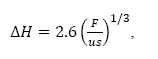
where u is the average wind speed, F is a flow parameter and s is a parameter of atmospheric stability.

where d represents the chimney diameter (in meters), T
0
the temperature (in Kelvin degrees) at the chimney exit,  is the environment temperature and V
0
is the gas speed (in m/s) at the chimney exit.
is the environment temperature and V
0
is the gas speed (in m/s) at the chimney exit.
The s parameter is calculated by the following eq. (2) found in [11]:
 (2)
(2)
where g is the acceleration due to gravity and  is the potential gradient of 0.02 K/m. This is chosen as default according to [5,19].
Values  and
and  were calculated experimentally by Pasquil and Gifford depending on the types of atmospheric stability. These results are summarized in [20]. However, due to the difficulty in obtaining exact data from the graphs, formulas have emerged such as the one developed by [21,22].
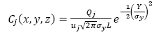
If the atmosphere is unstable or neutral and the value of the standard deviation in the 𝜎 𝑧 vertical plane is greater than 1.6 times the height of mixing, the concentration of the pollutant can be calculated according to [23] and using eq. (3):
 (3)
(3)
where L is the height of mixing.
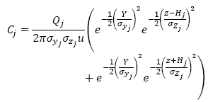
If atmospheric conditions are unstable or neutral where the value of is less than 1.6 times the height of mixing, the concentration is given by eq. (4):
 (4)
(4)
This series converges quickly and it is enough to take N values from -4 up to 4 [23].
It is important to reference Moses and Carson [24] who carried out experimental work in which they analyzed 711 plumes and found that Holland’s formula is well suited to sources with great heights.
2.1. Topography
When the surface of the region is not completely flat, the concentration of the pollution at each point may be different from that calculated by using any of the formulas 1, 2 or 3. For example, if a mountain ridge partially prevents horizontal dispersion, then the flow is approximately parallel to it. According to [20], assuming that the hill completely reflects the contaminant, then the concentration is calculated using eq. (5):
 ,(5)
,(5)
where B is the distance from the XZ plane to the hill when considering the positive Y axis in the direction of the mountain ridge.
The restriction of the horizontal dispersion generated by the existence of a valley is equivalent to that generated by the vertical dispersion by a layer of stable air. When is big enough and the distribution is approximately uniform, the concentration can be calculated by eq. (5, 17), as shown by Turner [20]. If the receiver is at a lower height than the source and the flow is parallel to the surface (of the mountain), then it is considered that there is no difference between the elevation of the floor with the receiver and with the source [20].
2.2. Reflection of the contaminant due to collision with the floor
If the floor is flat and the wind that carries the pollutant produced by a j source collides with it, a reflection phenomenon is generated, which makes the concentration at nearby points slightly larger. This increase is equivalent to the concentration generated by an imaginary source with a chimney of the same size as that of j, located symmetrically below the point where the actual source sits. In the Gaussian model, this phenomenon causes the appearance of a second exponential term.
If the surface of the earth is not perfectly flat, the collision does not occur at the same height z = 0. For the points of the floor that have a height that is less than the effective height of the source, the equation for the flat case can produce a concentration value lower than the actual value. To avoid this phenomenon, for each source in Ω, another virtual source is created that is symmetrical to the horizontal plane passing through the (x, y, z m ) point, at which the collision of the contaminant occurs. Thus, for a fixed source, its associated virtual source varies the height of the chimney depending on z m terrain elevation below the receiver section (x,y,z). The (x, y, z) point is located just above (x, y, z m ) on the same vertical line that passes through the (x, y, 0) point. This is incorporated into the model by subtracting the effective height of the elevation source from the z m surface below the (x,y,z) point where the concentration will be calculated.
The (x,y,z) point is located just above (x, y, z m ) on the same vertical line that passes through the (x,y,0) point. If we establish that Z = z - zm, i.e. Z is the height of the (x, y, z) point on the land surface in region Ω, then the concentration is calculated using eq. (6):
 (6)
(6)
2.3. Semi-infinite programming problem
If we consider pollution in a three dimensional area Ω coming from n fixed sources, then at each (x, y, z) point of Ω the concentration on the contaminant is 
 is the concentration provided by the j source and it is calculated using the formulas contained in the previous section, depending on meteorological and geographic conditions.
If w
j
(decision variable) denotes the reduction factor of the contamination for the j source when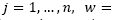
 , and assuming that the total cost G is a linear function of w
j
, then
, and assuming that the total cost G is a linear function of w
j
, then 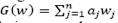 and the problem of minimizing air pollution control costs in Ω to fulfill with a φ rule is given in eq. (7):
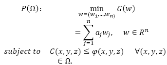 (7)
(7)
The considered problem has a finite (n) number of variables and an infinite number of constraints, as many as the number of points in Ω. These kinds of problems are called semi-infinite programming (SIP) problems and are an extension of classical mathematical programming. SIP allows the compliance of constraints to be observed at each control area point.
The optimal values of the w i variables indicate the contamination reduction percentages of each source i at the least cost.
In general, the  solution for an SIP is approximated by limiting solution successions
  for the finite sub problems P(Ωn) of P(Ω), so that Ωn→Ω when n→∞. There are various methods used to solve SIP problems, for example please see the work of [25-30]. The method used in this paper is one of the exchange methods. These methods have the advantage of not accumulating the active constraints but incorporating them by eliminating the previous ones.
2.3.1. The stochastic outer approximations method
To solve the problem P(Ω), we develop a version of Volkov-Zavriev´s [6] stochastic method of outer approximations. The convergence and applicability of this method is well studied, for example in the famous problem of Chebyshev's approximation.
Throughout this section we will denote, by using x = (x, y, z), a point in the  region, and the P(Ω) problem constraints will be written as g(w,x)≤0 with
  .
.
To establish the set of active constraints for each approximate problem, the algorithm must solve the local search problem for the maximum as shown in eq. (8):
 (8)
(8)
where w n-1 is the optimum of the P(Ω n-1 ) problem.
The approximate solution x for problem (8) is found by using the gradient projection method; x belongs to the stationary set as expressed in eq. (9):
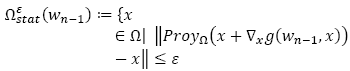 (9)
(9)
of the I.P. problem, that is to say, to the set of all the points that fulfill the necessary conditions for first order optimality, when ε > 0 exactly. The algorithm has two important parts:
2.3.2. Procedure SPROC.ACTIV.Medio.
Step 0. i = 1
Input parameters: 
Output parameters: 
Procedure parameters: δ>0, ε>0.
Step 1. Apply the local search algorithm (gradient projection algorithm) to solve the problem  starting from a random xi0 point in order to get
  point, so that
  and
and .
.
Step 2. Find  .
.
Step 3. If 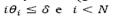 then i = i + 1 (
 is large enough), go back to Step 1.
Step 4. Stopping criterion of the algorithm, if i = N, perform  and exit.
Step 5. Perform .
.
2.3.3. The SMETH.ACTIV.Medio procedure
Parameters: ε, N, δ
Step 
Step 1. Find wn solution for the P(Ωn) problem.
Step 2. Call the SPROC.ACTIV.Medio procedure in order to get  .
.
Step 3. Stop if θn = 0
Step 4. Form a set of constraints

Step 5. n = n + 1, return to Step 1.
The algorithm ends when there are no more active points in Ω that do not meet the constraints of the feasible set of finite problems that were generated in the previous iteration. N represents the maximum number of searches carried out without any active points found.
To evaluate a point  as a local solution for the P(Ω) problem, the quasi-optimal function shown in eq. (10) is used (see [15]) :
 (10)
(10)
The quasi-optimal function plays the optimization criteria role for the SMETH.ACTIV.Medio method. Please note that if is a solution for P(Ω) problem, then  .
.
It has been shown that any trajectory of the SMETH.ACTIV method converges to the quasi-optimal set of the problem P (Ω) if the quasi-optimal function fulfills assumptions A1 and A2 as stated in [6]. Fedossova [31] demonstrated that the quasi-optimal function (10) does fulfill this hypothesis and, therefore, the SMETH.ACTIV.Medio method is a version of the SMETH.ACTIV method. Thus, any path of the SMETH.ACTIV.Medio method converges to the quasi-optimal set with a probability of one. To evaluate the quasi-optimal function there is no need to solve any additional problem [15]. This is an advantage of this version of the method used.
3. Results and Discussion
The method used to solve the problem of semi-infinite programming was implemented in MATLAB. Sulfur dioxide (SO2) was chosen as the contaminant since it has been previously studied in many regions of the world such as Turkey [32], China [33] and Mexico [34], the last country being the closest to the Colombian environment in terms of location and industrial practices. Bogotá, the capital city of Colombia, has a concentration limit standard for this pollutant that is 250 x 10-6 g/m3 [22]. The formulation of the cost minimization problem of air pollution control in region Ω with ten sources is given in eq. (11):
 (11)
(11)
The problem scenario includes a mountain in region Ω, and it is assumed that we know with good precision the elevation of each of its points. The algorithm used to obtain the constraints of the P (Ω) problems does not consider the points below the mountain surface as possible points for the parameters set.
The sources are located based on Wang and Luus [35], and correspond to the first two columns in Table 1. For instance, source 6 with plane coordinates (22700, 21000) is situated on the mountain at a height of 400 m. A panoramic of the sources placement for this problem can be observed in Fig. 1.
Results presented in the numerical results section have been obtained for different considerations of Ω. We considered three cases, two include the phenomenon generated by the collision of the contaminant with the surface, also known as reflection. In all cases, it is assumed that the wind speed is 5.637 m/s in a θ=3.996 (rad) [35] direction.
3.1. Numerical results
Case 1:  with reflection.
We used W0 = (0, 0, 0, 0, 0, 0, 0, 0, 0, 0) as the starting point. The approximate cost of pollution control obtained in 50 iterations was 5.9534. Table 2 shows the percentages by which each source must be reduced at the least cost.

The finite subset that generates the constraints is determined by the SPROC.ACTIV.Medio procedure. Each constraint is obtained using eq. (11):
 ,(12)
,(12)
where  , is the j-th row of the matrix of sub problem constraints that approximates the original constraints set.
The evolution of the pollutant´s reduction factors for each of the sources, along the algorithm iterations and starting at W0, is shown in Fig. 2. Although Fig. 2 shows that the reduction factors behave as monotonous functions, this phenomenon may generally not occur because the whole set of constraints is being modified at every step.

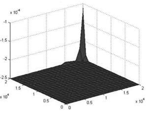
The g(w,x) is the difference between the concentration and the norm and verifies that the constraints are being met. The results for floor level and the plane at a height of 100 m are shown in Figs. 3 and 4, respectively.
Please note that at surface level  , while at a height of 100 m, there are points where
  . This is to be expected if we consider that these points are closer to the effective height of the chimney.
Source: The authors
Figure 3 Difference between the concentration and the norm (g/m3), on the surface (after the reduction).

Source: The authors
Figure 4 Difference between the concentration and the norm, in z = 100 m, after the reduction.


Case 2: Ω=[0,40000]×[0,40000], on the surface.
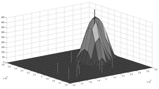
This case assumes that Ω=[0,40000]×[0,40000]. The environmental standard is 350 g/m3 and the effect of reflection due to the impact of SO2 on the surface is taken into account. The approximate solution for the problem was obtained in 27 iterations and is presented in Table 3. For this case W 0 = (0, 0, 0, 0, 0, 0, 0, 0, 0, 0) was chosen as a starting point and the distribution of sources is identical to the previous sections. The subset Ω27, from which we generated constraints for the P Ω27 problem, provides us with a solution that allows us to approximate one for the original problem. This is shown graphically in Fig. 5.
The value of the cost function at the optimal point is 7.7922, i.e. it is the same scenario as described above. The lowest cost to reduce emissions, so that the concentration is less than 350 g/m 3 , is 7.7922 times the monetary value of reducing one percentage unit.
Case 3: Ω=[0,40000]×[0,40000] x [0,400], with reflection.
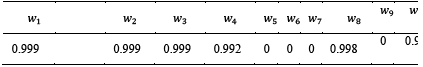
The reduction factors 𝑤 𝑗 , which produce the least cost, are given in Table 4.
To verify that the result satisfies the constraints, the problem was solved when w i , j =1, …,10 corresponds to the values in the table above.
The highest value for the concentration of the contaminant that is obtained using a grid with a 50 m horizontal size and a 10 m vertical size is 84.93 x 10⁻⁶ and it occurs at point (22200, 21000, 320).
It is important to compare the results obtained in cases 1 and 3 that include a mountain. For case 1, some sources have been left outside the area of control, and the height of the control region has been reduced in order to ensure that the effective heights from all sources are outside the region. In this case, compared to case 3, none of the sources must fully reduce emissions. In addition to the sources that are not within the control area, only source 10, which is the closest, must reduce its emissions.
In both cases 1 and 3, the points with the highest concentrations of the pollutant after reduction are at a significant height. In case 1, the points with a pollutant concentration very close to the allowed limit are found at 100 m above surface level. Meanwhile, in case 3, the point with the highest concentration was located at 320 m, well above the heights of chimneys.
4. Conclusions
In this paper we have used a Gaussian model to calculate the concentration of a pollutant, and we have carried out numerical experiments for sulfur dioxide, using real parameters. In some cases the Colombian standard of 250 x 10-6 at an environmental temperature of 25ºC was applied.
In the scenario used for the numerical experiments, a mountain was introduced (for the first time) with a maximum height of 400 m. The effects that are generated as a result of locating a source there are captured by the plume elevation and the dispersion measurements. When we deal with greater height the wind has less friction, and, in addition, the amount of atmosphere available for dilution of pollutants is higher.
To solve the problem of semi-infinite programming, the stochastic method of outer approximations was applied [6]. The algorithm was implemented in MATLAB. According to the results, the sources located within the region where the standard has been established should reduce over 90% their current emissions. These results are aligned with the hypothesis that fixed sources of contamination should not be set within cities. They are also consistent with the fact that environmental standards are differential in industrial areas. By applying the model to future scenarios, the solution allows researchers to estimate the effects that are generated by establishing a source in a specific area and establishing its effects on the environment.

