Introduction

Over the years, the world economy has oriented its markets towards globalized supply and demand. In the case of Colombia, this process started in the 90s with the beginning of the economic opening, when new competitors were allowed to enter the market, many of which were foreign producers. Due to this situation, several economic sectors disappeared, as it was not possible to compete with the wide range of products and prices in offer ^{(1, 2)}.

In light of the above, a large number of international companies entered the Colombian market, especially in the retail sector, which represents 56 % of retail sales. Within this business paradigm, large sales chains such as Éxito, Carrefour (today Jumbo), Carulla, Olímpica, Super Inter, and Makro stand out. These companies assess the procurement of supplies based on efficiency indicators, aiming to maximize the return on investment. However, there is a second model that concerns the neighborhood convenience stores of the traditional channel. The most noticeable difference between these two models corresponds to administration, which is carried out by the owner or head of the family unit in the second case ^{(1, 2)}.

Despite stiff competition, neighborhood stores have survived due to their closeness to the final consumer, their trust and empathy with customers, and the payment methods offered (interest-free credit). Neighborhood stores have been hit hard by the advent of large discount store chains, such as ARA, D1, and Justo & Bueno, which aim to get closer to the end customer and compete with low prices ^{(3, 4)}. Therefore, the traditional channel in Colombia must improve, update, and transform its processes, specifically in making decisions on the projection of supply and demand, as well as in inventory rotation ⁵.

In general terms, the store administrator manages the investments in the purchase of the products offered according to their expertise and knowledge acquired from the market. It should be stressed that this is a subjective forecasting method based on experience. This strategy generates a high bias in facing the uncertainties presented by changes in the demand for certain items according to the season and the economic variations in prices, state policies, and social events ⁶.

Likewise, it has been identified that demand forecasting is a common problem in supply chains. Here, the objective is to achieve greater precision and less error. According to ⁷, given the diversity of demand patterns, it is unlikely that any single demand forecasting model can offer the highest accuracy across all items. On the other hand, managers frequently have more information that should be considered to improve forecast results. For example, they know customer habits and purchase intentions, among others ⁸. A better forecast should include all this information. However, this requires more advanced methods than those offered by the prediction techniques of machine learning.

Considering the above, artificial intelligence (AI) and machine learning techniques have been proposed in the literature, aiming to reduce bias and provide business units with decision-making tools under a data-based paradigm, largely because AI models allow them to carry out forecasting with regard to the demand for items ⁹. In the state of the art, two major stages are identified in which these procedures are focused. The first involves collecting and characterizing the data, with the purpose of describing the behavior of the products and its variability over time. In the second stage, different machine learning techniques are used to estimate computational models that can predict and reproduce the dynamics of the data, so that the sales dynamics can be emulated over time for a set of specific items ^(10-13).

Usually, the forecast of pure units or goods follows a uniform or normal probability distribution ¹⁴. More specialized developments introduce planning aspects that drive the supply chain as customer expectations increase, shortening delivery times, and pressure for resource optimization ¹⁵. On the other hand, demand forecasting is generally carried out using machine learning techniques. An example of this is the use of neural networks, which emulate the forecast of items through a non-linear function in time. Historical sales data are included in the network design in combination with the effectiveness of advertising, promotions, and marketing events. However, this model is sensitive to the network architecture (i.e., the number of hidden layers and the value of neurons per layer), which affects the generality of the method ¹⁶. Other methods also predict demand, such as the Auto Regressive Moving-Average (ARMA), Support Vector Machine (SVM), Multiple Linear Regression (MLR), and Random Forest models, showing competitive results adjusted to reality. Still, this approach predicts the quantities of products required without considering the investment and profit capabilities of the shopkeeper ^{(17, 18)}. Other works demonstrate the application of chaotic methods, such as ^(19-21), achieving demand adjustment.

As of today, the sudden changes in the market have generated new paradigms of competition. These circumstances are experienced by emerging businesses such as neighborhood stores ²². Studies such as ²³⁾ show that more than 90 % of the data generated by these businesses are not exploited and are not used to make sense of the changing dynamics of the market. There are success stories where machine learning has been used to better predict and manage expenses ²³. This optimizes business profits, thus allowing for small businesses’ economic survival. Some sources claim that including these methodologies can add significant value to their demand forecasting processes, while more than half state that they can improve other eight critical supply chain capabilities ²⁴.

The above-mentioned study added that retailers with the technology to predict these changes model contingency plans and options and quickly adapt their supply chain strategy to meet high demand and avoid excess inventory. Those who cannot do it risk falling behind with sales not meeting the goals, in addition to incurring losses through waste ²³. This research describes and structures a methodology for forecasting the quantities needed to order certain products in neighborhood stores. The method proposes a linear model to maximize the shopkeeper’s profits based on an available investment value that, combined with a machine learning procedure, allows inferring the amounts to be requested. This method constitutes an alternative detached from the traditional paradigm of neighborhood stores, which is built daily and considers the last order requested, ignoring the behavior in sales and the dynamics of customers ²⁵.

This proposal employs three models for sales forecasting, i.e., the performance of an SVM, a Gaussian process (GP), and an ARx model are examined using synthetic data generated via statistical sampling according to the Probability Distribution Function (PDF) that is accentuated to the sales of the products under analysis. The selection criteria for the PDFs of the products studied are in accordance with ¹⁴, which suggests using uniform or Gaussian PDFs for products offered in neighborhood stores. Additionally, the methodology proposes error metrics and statistical analysis to evaluate and validate each of the models selected in this research. The results show that our proposal allows maximizing the shopkeeper’s profits by considering the dynamics in sales and the available investment. The main contributions of this research are the following:

This paper is organized as follows. Section 2 presents the basic nomenclature. Section 3 describes the proposed methodology, as well as the validation procedure, and the results obtained are shown in section 4. In the final section, the concluding remarks of our research are presented.

Basic nomenclature

Table I Paper nomenclature 

Methodology

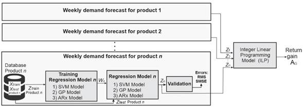
Fig. 1shows the implemented method in a block diagram. In short, it consists of three phases: firstly, a database with information on the demands per week for 14 everyday items offered in neighborhood stores; secondly, a regression model that emulates the prediction Z = {Z ₁ Z ₂ . . . Z _n }, where Z _n is the prediction of the n-th product; and, finally, an integer linear programming model that refines the weekly orders to maximize the profit return A _G given a weekly investment rate. Traditionally, inventory management models include a systematic methodology to establish inventory control policies for products. This allows determining the security list, the reorder point, or when the order must be placed ^26). This research aims to reduce the overall costs by predicting the demand for key products in neighborhood stores. It analyzes projected profits based on the model’s predictions. It must be acknowledged that this study does not encompass all aspects of defining inventory control policies.

Figure 1 Implemented methodology 

Database

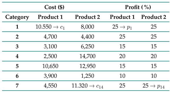
In this study, seven categories that cover 14 product varieties in neighborhood stores were selected, as summarized in Table II. Each product is independent, so all analyses are proposed and done for each one of them.

Table II Selected categories and products 

This selection was done by visiting shopkeepers in neighborhoods of Pereira (these items were selected since they were representative of the sales during the analyzed time horizon) and identifying common items such as those shown in Table II. Additionally, the variability in their demand was validated, finding that some exhibit a temporary behavior, as is the case of category 6 (products of great demand on celebration dates, i.e., holidays, commemorative days, among others).

Conversely, other items show a stable behavior over time, as is the case of the products in categories 5 and 7. The literature states that the demand follows a certain PDF, which, in the case of basic products, can be adjusted to a normal or uniform behavior ²⁷. Due to the above, it is possible to generate synthetic data from a statistical sample while assuming a PDF for each category, establishing the distribution parameters for each item ( Table III).

Table III Definition of the model for data generation 

The expected values u _Y (where Y is the weekly demand) and the standard deviation σ _Y of the distribution given in Table III, are summarized in Table IV. The first moments for a normal and uniform distribution are u _Y = µand , respectively. Similarly, the variance in the case of a Gaussian and uniform PDF is σ _Y = σ and ¹⁴.

Table IV Expected values and distributions from Table III 

Thus, the demand per week (for each product) was sampled over a time window of 78 weeks, i.e., the data generated emulate the dynamics of the demands per product for this sales interval. Once the database was formed, it was segmented as follows: X = {X _{T rain} , Y _{T rain} , X _{T est} , Y _{T est} }. Then, a characteristic was added to the vectors X _{T rain} and X _{T est} which models the increase or decrease in the number of requested units of a product with respect to the previous week. Eq. (1) shows the transformation for the Y _{T rain} case, following a similar procedure for Y _{T est} .

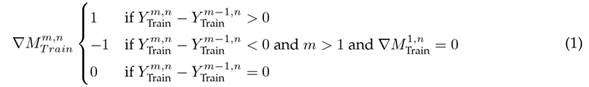
The sub-index m refers to the analyzed week for product n (defined in Table II). Eq. (1) indicates that, if the value of , there was an increase when ordering product n in week m regarding the m − 1 period. On the other hand, a value of implies a stable behavior in week m regarding the moment m − 1. This descriptor seeks to guide the learning model at the moments when changes occur in the demands of the n products. For more details, the reader should consult (28). With these changes, the terms are defined as follows:

Model training

Fig. 2 shows each of the stages that make up the training phase. In short, it consists of a database that integrates synthetic data of demands per week for a family of products, as well as a supervised learning model to emulate the dynamics of weekly demands. The purpose is to transfer the data content to the model through a learning rule that allows finding the set of parameters W _n .

Figure 2 Prediction model diagram 

Supervised learning model

In this paper, three supervised options for state-of-the-art training are examined. Each of these is described below.

SVM

The use of an SVM as a prediction model is mainly due to its robustness against data with noise. It is a widely studied method, and it is easy to implement. This method is characterized by being a linear model in the W _n parameters, which are tuned by minimizing a regularized error function subject to a set of linear constraints.

Generally, the problem is usually transformed into an equivalent dual one by applying the KKT (Karush-Kuhn-Tucker) conditions, obtaining a quadratic representation that allows the value W _n to be inferred when it is solved. Once the parameter values W _n are known, the model is trained. However, the equivalent objective function will depend on some variables assumed to be known, such as the Z _{T rain} data set, as well as the Kernel structure (covariance function) ^{(29, 30)}.

ARx Model

The acronym ARx refers to an autoregressive model of exogenous terms. It involves an input signal in its structure. Eq. 2 shows this model. The meaning of each term is shown in Table V.

Table V Nomenclature associated with the ARx model 

The set of parameters to infer W _n corresponds to the set of values of the coefficients a _n a and b _n b . These are tuned via least squares through the Z _{T rain} dataset. Then, once the values of W _n are known, the model is determined for any value of t, assuming that W _n is known. For more details, the reader can refer to ³¹.

Gaussian process (GP)

Contrary to previous methods, the GP introduces a probabilistic non-linear prediction function, preventing a fixed structure in the model. From its base, the model assumes that the nature of the data follows a Gaussian distribution function established by a mean function m(x) and a covariance cov(x, x). In the literature, cov(x, x) is also known as Kernel, so the model training consists of tuning the parameters of m(x) and cov(x, x) (i.e., W _n ) given the input X _{T rain} and output Y _{T rain} (Z _{T rain} ) dataset. The prediction process (once the model has been trained) is performed from the mean predictive function, as shown in Eq. (3).

where m ^′ (x ₁) is the prediction in space x ₁ given the input x and the corresponding output y. An interesting feature of the GP allows computing the evolution of uncertainty (Eq. (4)) in the prediction using the predictive standard value (Eq. (3)), where σ(m ^′ (x ₁)) evaluates the uncertainty (variance) of m ^′ (x ₁). The GP implicitly assumes that the function m ^′ 1(x ₁) obeys - as does m(x) − a Gaussian behavior ³².

Validation

In this process, the performance of the trained models is evaluated through the dataset (X _{T est} , ∇M _{T est} ) and the corresponding prediction Z (Fig. 2). In the first place, the effective error is used as a performance metric (Eq. (5)) where E is the RMS error between the synthetic data validation vector and the prediction of the model ³⁰. Here, N refers to the size of the vector Y _{T est} .

This metric allows evaluating the fidelity of the trained model to emulate the prediction process of product demands. However, the Y _{T est} and Y _{T rain} data must be normalized to avoid bias regarding strong changes. In this work, they are normalized with respect to the mean value of the data as follows: A similar transformation applies to Y_{T rain}. Thus, Eq. (5) is transformed into the following expression:

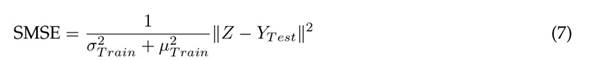
On the other hand, Eq. (7) defines the form of the standardized mean squared error (SMSE) (33):

where and µ _{T rain} are the variance and arithmetic mean of the Y _{T est} data. The metric given in Eq. (6) has the purpose of evaluating the stability of the prediction model Z when considering changes in the training data Z _{T rain} .

Integer linear programming model (ILP)

Z is an expected value of the demand. However, the shopkeeper will not always have sufficient resources to meet the quota established by the prediction model, which is why a strategy that refines the suggested Z values through a linear optimization model is adopted. The objective function to be minimized is presented in Eq. (8).

where Z ^∗ = (Z1∗, Z2∗, . . . , Z1∗4) are the quantities demanded weekly to be refined for each of the items defined in Table II, and P = (p ₁ , p ₂ , p ₃ , p ₁₄) denotes the corresponding percentages of profit from the sale of each product. The restrictions associated with the maximum number of items allowed are as follows:

where Z ^m,n refers to the predictions of item n(n: 1 : 14) for week m. Therefore, Eq. (9) yields 28 linear constraints given a value of m. Finally, the equality associated with the investment in week m is

where C = (c ₁ , c ₂ , c ₃ . . . , c ₁₄) are the purchase costs per item. Now, the refined quantities Z ^∗ are found by solving the following ILP problem (Eq. (11)) for an investment G associated with week m.

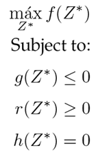
Note that the presumption of solving the problem stated in Eq. (11) is due to the fact that the quantities to be refined have a discrete characteristic. The values of P and C have been extracted from the portal www.megatiendas.co, and they are condensed in Table VI.

Table VI Definition of the values for the percentage gain vector P and the cost per product C 

Experiments

The test procedures evaluated the performance of the learning rules and the ILP. For the first case, the performance of the three strategies was evaluated by computing the values of E and SMSE (Eqs. (6) and (7)) for the prediction Z produced by the model and the test dataset Y _{T est} . Out of the 78 weeks, the first 55 were selected with their corresponding demands to build the vectors X _{T rain} , Y _{T rain} , and ∇M _{T rain} . Then, with the other weeks (56 to 78), the validation array X _{T est} , Y _{T est} , and ∇M _{T est} was made. The test in Algorithm 1 shows the process that summarizes the above.

For the case of GP and SVM, a radial basis covariance function (RBF) with scale factor ρ ² was assumed (32). This parameter was tuned given the Z _{T rain} dataset. The GPML (34) toolbox was used to train (find W _n ) and validate the GP (the value of ρ ² was also tuned with this toolbox). For the SVM, MATLAB’s regression toolbox in MATLAB was employed. In this case, a value of τ ² = 0, 001 (length scale) was set for the tests. The results are presented by means of tables and figures depicting the behavior of each model. In the case of the GP, the results are based on Eqs. (3) and (4). Finally, based on the results, the best prediction model was selected in order to evaluate the performance of the ILP.

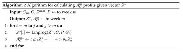
The experiments carried out in the ILP consist of validating the problem stated in (11). For this purpose, weekly test investments G _m , are defined. Thus, the refined quantities Z ^∗ are calculated given the weekly investment G _m and Z ^m,n . Finally, the expected return earning rate A _G is calculated according to the suggested amount Z ^∗ by the model in week m (Eq. (11)). Algorithm 2 shows a summary of the refinement process of the quantities Z and the profits for each of the weeks m under analysis.

Results

This section presents the analysis and discussion of the results obtained by implementing the methodology and performing the validation tests proposed in the methodology section. Fig. 3 shows the demand estimation made via the proposed prediction methods for product 14. In 3c, it can be seen that the ARx is the predictor that manages to capture the trend of the data and the demand variability for the item in the time window.

Fig. 3b shows GP’s low performance, as it fails to predict the variability of the demands when estimating an average value. Although the SVM manages to improve the prediction concerning the GP, this variation is not enough to emulate the dynamics of the weekly demands of the products (Fig. 3a). The quantitative results are shown in Fig. 3b. The results regarding the effective errors are condensed (Eq. (5)) once the Monte Carlo experiment has been simulated (Algorithm 1). As per Fig. 4b, the ARX shows a lower error when compared to the SVM (Fig. 4d) and the GP (Fig. 4f), which corroborates the results shown in Fig. 3. It is noteworthy that the minimum error for the training demands is reached by GP (Fig. 4e). This suggests that the model is overtrained, which explains the result in Fig. 3b. On the other hand, Fig. 4d shows that the SVM responds adequately to products with low variability, as is the case of the items in categories 1 and 7 (Table II).

Figure 3 a) Demand estimation using the SVM method. b) Demand estimation using the GP method. c) Demand estimation using the ARX method 

Figure 4 a) Training RMS error for the ARX method. b) Test RMS error for the ARX method. c) Training RMS error for the SVM method. d) Test RMS error for the SVM method. e) Training RMS error for the GP method. f) Test RMS error for the GP method 

Fig. 5 synthesizes the results for the SMSE metric. The GP fails to stabilize in the training phase regarding the categories {1,2,7, 12, 13}. On the other hand, the SVM and the ARx exhibit a similar qualitative behavior in all the product categories under study, both in the training stage and during the validation. The results suggest that the prediction computed by the three methods evaluated is stable. This corroborates what is evidenced in Figs. 5 and 6, where the change in the datasets Z _{T rain} and Z _{T est} fails to capture the dynamics of the data, nor does it significantly reduce the effective errors, mainly in the case of the SVM and the GP. The above insinuates that they fail to satisfactorily emulate the behavior of the demands. This may be due to the nature of the application, where the analysis time window (104 weeks) is restricted for these models.

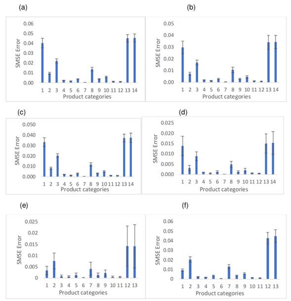
Figure 5 a) Training RMS error for the ARX method. b) Test RMS error for the ARX method. c) Training RMS error for the SVM method. d) Test RMS error for the SVM method. e) Training RMS error for the GP method. f) Test RMS error for the GP method 

Table VII summarizes the results obtained by calculating the first expected value and the variance of the predictors for each of the studied products’ demands. The ARx manages to approach the theoretical statistics, which is a significant result, suggesting that it manages to capture the variability and the mean value of the distributions associated with each of the demands. However, although the SVM and the GP approach the first theoretical moment of the data, they fail to capture the variability; these predictors have a variance bias in this application.

Table VII Results regarding the expected value and variance for each of the predictors 

Given that the ARx exhibits a good performance in estimating the demands in each of the categories, and considering that the SVM and GP do not reach competitive performances (Table VII, Figs. 3, 4, 5), the outputs Z inferred by the ARx are selected to build the integer programming model described in Eq. (11) in such a way that it is possible to refine the quantities Z by defining a weekly investment index to determine Z ^∗. Fig. 6 shows the difference between the profits when considering a sufficient investment to acquire the amounts Z versus the profits gained when examining a smaller investment to obtain Z ^∗ in a cumulative period of 22 weeks. Notice how, in the linear programming method, the profits approach the maximum values as the investment grows. This is an expected result since the formulation aims to provide further weight to the products with the highest profit; the method suggests the amounts that maximize profit to the shopkeeper. It should be noted that, from an investment of 1.200.000 COP, it is possible to obtain the same profit as the one obtained with the Z amounts, i.e., the values suggested by the ARx.

Figure 6 Difference between the profit projected by the estimation of the product and the profit obtained by the integer programming model for 22 weeks of analysis 

Fig. 7a shows the expected profit for 22 weeks according to the amounts Z.It also shows the profit for the amounts Z ^∗ corresponding to an investment of 1.220.000 COP. This shows that the linear programming model does not affect the trend of expected profits. Note that this result is still valid for smaller investments (Fig. 7b), and it is important because the method guarantees proportionality in profits, even if the investment is low.

Fig. 8 shows how the solution to the problem given by Eq. (11) refines the number of products and prioritizes those that generate greater profits. For example, in Fig. 8a, the model gives priority to products 1, 2, 3, 4, 13, and 14 when comparing them against the utility portions defined in Table 7. They coincide with the items that report the highest percentage of utility per sale. Similarly, it should be noted (Fig. 8b) that, as the investment value increases, the amounts Z ^∗ tend to equal the values of Z, which corrects the results reported in Figs.6 and 7.

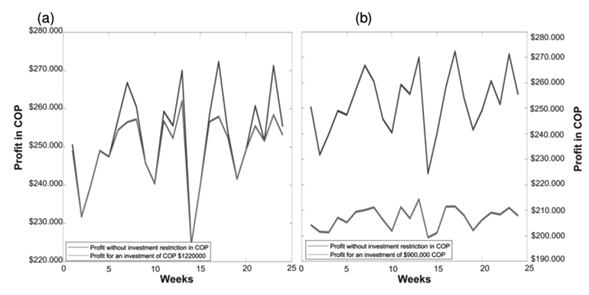
Figure 7 a) Expected profit with Z vs. profit obtained with Z ^∗ for 22 weeks, corresponding to an investment of 1.220.000 COP. b) Expected profit with Z vs. profit obtained with Z ^∗ for 22 weeks given an investment of 920.000 COP 

Figure 8 a) Estimated amounts for the 14 products in 22 weeks vs. refined amounts for a weekly investment of 500.000 COP. b) Estimated amounts for the 14 products in 22 weeks vs. refined amounts for a weekly investment of 1.000.000 COP 

Conclusions

In this research, a methodology is designed and implemented with the aim of estimating the demand for products sold in neighborhood stores. This is achieved based on the history of the weeks of sales for previous months and weeks. This method estimates demand and suggests which products to buy in order to maximize profit based on an available investment cost. Based on the results, it is observed that the model proposed in Eq. (11) is functional to the extent that the investment available per week is not sufficient to acquire the amounts Z. This is inferred by analyzing that reported in Figs. 8a and 8b, where the behavior of the amounts Z and Z ^∗ is described as an investment value. The aforementioned is an expected result because, at a higher level of investment, the amounts Z ^∗ are closer to Z. Therefore, it is concluded that the refinement process of the proportions of Z becomes unnecessary at high levels of investment.

On the other hand, the results show that, for this application, the ARx is the model that is closest to the data dynamics (Table VII), managing to reproduce the first moment and the variance of the probability distributions assumed in Table III. This is verified by analyzing the values of the effective errors reported in Fig. 4b, where the ARx proves to be more competitive than the SVM and the GP.

The differences per product regarding the behavior of the effective error for the studied learning models can be explained by analyzing some categories’ variances. For example, from Table IV, items 11 and 12 have a high variability concerning the others, i.e., they exhibit a greater range of fluctuation in demand. Note that, in these particular cases, the effective error is significantly higher when compared to products with low variability, as for those belonging to category 1. The above suggests that the prediction models’ yields are sensitive to solid changes in demand.

As further work, the proposed method must incorporate other relevant variables, allowing for qualitative and/or quantitative variables to be weighted in order to refine the Z quantities. This is essential, given that, in a competitive environment such as the neighborhood grocery store market, the supply of different products should not be strictly conditioned as being a problem of maximizing the shopkeeper’s profits according to the items that yield the highest profit. However, on the contrary, it should consider the client’s needs, so that these are incorporated into the strategy for calculating Z ^∗. On the other hand, it is also important to validate this methodology with different neighborhood stores, as well as to measure the possible impact of the methodology, for it is imperative to build software that allows the shopkeeper to manage it with ease. This information can be valuable to grow the model and thus correlate other variables currently unknown to the method