


 Inglês (pdf)
 Artigo em XML
 Referências do artigo
 Enviar este artigo por email
 Citado por SciELO
  Citado por Google
  Similares em
SciELO
Similares em
SciELO  Similares em Google
 Permalink
1. Introduction
The heat equation, which is the mathematical model for heat flow, and in its simplest form is written as

where Δ is the Laplace-Beltrami operator, is among the most relevant partial differential equations in mathematics and physics, and it has truly remarkable properties. For instance, if an "arbitrary" initial condition f
0
is subjected to this equation, then the solution f
t
, for any instant of time t > 0, will be a  function. In the light of such facts, the heat equation presents itself as a fundamental smoothing process.
In a recent paper [7], a result in this direction was established, further evidencing important smoothing properties of this equation. Given a smooth function f defined on a manifold M, an indicator of regularity for f is whether all of its critical points are non-degenerate, which is to say that f is a Morse function. The authors showed (see Theorem 2.1 and Theorem 3.1 of that paper) that, at least in the case of n-dimensional round spheres or flat tori, "arbitrary" smooth initial conditions fo are eventually transformed by the heat equation into minimal Morse functions; Morse functions that have the smallest possible number of critical points in the manifold.
Investigating the question of whether this is a more general phenomenon presenting itself in other compact Riemannian manifolds, this paper presents proof of the analogous result for real and complex projective spaces of arbitrary dimension. We will further observe that in these spaces, the heat process endows the solution ft with a fundamental property called stability, which roughly speaking means that functions close to ft will be "identical" to ft modulo a suitable change of coordinates.1 This is made precise by the following definition.
Definition 1.1. Let M be a compact smooth manifold, and let . f is said to be stable if there exists a neighborhood Wf of f in the Whitney
  topology such that for each
  there exist diffeomorphisms g, h such that the following diagram commutes:

The corollary to the following fundamental theorem (see [4, pp. 79-80]) gives a simple characterization of stable functions which will be key to what follows.
Theorem 1.2 (Stability Theorem). Let M be a compact smooth manifold, and . Then f is a Morse function with distinct critical values if and only if it is stable.
Corollary 1.3.
If M is a smooth compact manifold, and f is a Morse function with distinct critical values, then there exists a neighborhood of f in the
 topology such that g is a Morse function with distinct critical values and the same number of critical points as f for all g in said neighborhood. In particular, since M is compact (so that the topology has the union of all
  topologies as a basis, each a Banach space [5]), there exist r and Є > 0 such that g is a Morse function with distinct critical values and the same number of critical points as f whenever
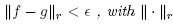 being a fixed norm for the
  topology.
Now, our precise formulation of an "arbitrary" smooth initial condition f
0
will be that it belongs to a fixed open and dense set S in the topology. We can now state the two main results.
Theorem 1.4. There exists a set  , that is dense and open in the
  topology, such that for any initial condition
  is the corresponding solution to the heat equation on
 at time t, then there exists T > 0 such that for t ≥ T, ft is a stable minimal Morse function on.
Theorem 1.5. There exists a set  , that is dense and open in the topology, such that for any initial condition
  is the corresponding solution to the heat equation on
  at time t, then there exists T > 0 such that for t ≥ T, ft is a stable minimal Morse function on.
The basic strategy for the proof on both spaces may be sketched as follows: On compact Riemannian manifolds, as is well known, the solution has the form
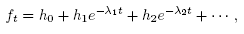
where  are the eigenvalues for the Laplace-Beltrami operator, and the hi are the projections of f
0
onto the corresponding eigenspaces. The overall idea is to exploit the exponentially decaying terms of the solution to approximate f
t
by the first two terms of the sum for large times. Our set S will then consist of those functions for which said first two terms add up to a stable, minimal Morse function. Since stability is by definition a property unchanged by small perturbations, it is apparent that the desired result follows provided that
are the eigenvalues for the Laplace-Beltrami operator, and the hi are the projections of f
0
onto the corresponding eigenspaces. The overall idea is to exploit the exponentially decaying terms of the solution to approximate f
t
by the first two terms of the sum for large times. Our set S will then consist of those functions for which said first two terms add up to a stable, minimal Morse function. Since stability is by definition a property unchanged by small perturbations, it is apparent that the desired result follows provided that
(i) S is dense and open, and
(ii) we successfully bound the remaining terms to make the approximation work.
In section 2, simple conditions for the main result to hold in a manifold will be established, as well as a technical statement that will be needed later to verify the above-stated conditions on the two spaces in question. On the other hand, sections 3 and 4 are, respectively, dedicated to the proofs of Theorems 1.4 and 1.5.
2. Basic results
The following lemma gives two concrete sufficient conditions for items (i) and (ii) of the introduction to be true, and thereafter makes rigorous the previously sketched strategy to prove (using some simple estimates and the profound characterization of stability given by Theorem 1.2) that the desired theorem will follow on compact Riemannian manifolds in which the eigenvalues grow at least linearly as soon as we have these two sufficient conditions.
Lemma 2.1.
Let
M be a compact, connected Riemannian manifold, let
 be the distinct eigenvalues for the Laplace-Beltrami operator and let
  be any basis (not necessarily orthonormal) for the
  -eigenspace. Suppose the eigenvalues grow at least linearly,2 that the 0-eigenspace is trivial,3 and the following two conditions hold:
(C1) The set B of d,1-tuples ( ) such that
 is a minimal Morse function on M with distinct critical values is an open dense subset of
 .
.
(C2)
For each
 , there exist N, C such that the projection
 of f onto the j th eigenspace satisfies

Then there exists a set , that is dense and open in the
 topology, such that for any initial condition
  is the corresponding solution to the heat equation on M at time t, then there exists T > 0 such that for t ≥ T, ft is a minimal Morse function with distinct critical values on M.
Proof. Let S be the set of functions f whose projection  onto the
  eigenspace is a minimal Morse function with distinct critical values. Let f Є S. By compactness,
  , so functions in a sufficiently small neighborhood U of f in the C0 topology (which is contained in the
  topology) will have its Fourier coefficients (with respect to any fixed orthonormal basis) as close as desired to those of f. Observing that the coefficients with respect to
  are continuous functions of the Fourier coefficients for the
  eigenspace, condition (C1) implies that if U is small enough, U C S, hence S is open. Now let
  , and let g be obtained from f such that
  and
and  comes from slightly modifying the coefficients of
  with respect to
  so that is a minimal Morse function with distinct critical values (this is again possible by condition (C1)). By compactness of M, if the modification is slight enough, g will be as close as desired to f in any C
r
(and so in the
so that is a minimal Morse function with distinct critical values (this is again possible by condition (C1)). By compactness of M, if the modification is slight enough, g will be as close as desired to f in any C
r
(and so in the  ) topology. So S is dense. Now we check that if f Є S and
  with
with  , then
  is Morse minimal with distinct critical values for large enough t. Since h
0
is constant it suffices to show the same for
is Morse minimal with distinct critical values for large enough t. Since h
0
is constant it suffices to show the same for , and by Corollary 1.3 it is enough to prove that for each r,
  One has

Because the  grow at least linearly, the series on the right is clearly convergent and a decreasing function of t, and the first factor tends to zero as
 , so this completes the proof.4

Since the real and complex projective spaces, besides conditions (C1) and (C2), are easily seen to satisfy the hypotheses of the above lemma,5 the remaining major part of this paper is dedicated to proving that the aforementioned conditions do hold on these spaces, from which the theorems will follow. We end this section with a technical statement that will be needed later for this purpose.
Lemma 2.2. Let M be a smooth manifold and let G be a Lie group acting smoothly, freely and properly on M. Let  be constant on each G-orbit, so that it descends to
 . Then there exist smooth coordinates (
 ) for M such that (
 ) are coordinates for M/G and
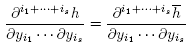
for any indices i 1,…, is.
Proof. In Theorem 21.10 of [6] one sees that there exist cubic coordinates(  ) for M that intersect each G-orbit in either the empty set or a slice (
 ) = (c1,..., ck) and such that(
 ) are coordinates for M/G. In these coordinates it is clear that

and the statement follows by differentiating both sides 
3. Real projective spaces
In this section we demonstrate our result for real projective spaces . By construction, the space of functions on (realized as
 , with G being the two element group generated by the antipodal map) is identified (via pullback) with the functions in S
n
for which
, with G being the two element group generated by the antipodal map) is identified (via pullback) with the functions in S
n
for which

Therefore, one sees that the eigenfunctions for the Laplace-Beltrami operator in this manifold are precisely the ones on S
n
that satisfy f (x) = f (-x). That is, the eigenvalues are  , with the corresponding eigenspace being the space of homogeneous harmonic polynomials of degree 2k in n +1 variables [2]. The following proposition is then a detailed analysis of the first non-trivial eigenspace, whose ultimate purpose is the verification of condition (C1) of Lemma 2.1.
Proposition 3.1. Let  be a real quadratic form in n +1 variables, with A = (
 ) being a symmetric matrix.6Then f is a minimal Morse function on
 with distinct critical points if and only if the matrix A =(
 ) has distinct eigenvalues.
Proof. We may diagonalize this quadratic form through an orthogonal change of coordinates y = Bx, and write  where
where  are the eigenvalues of A. Write
  . The gradient of f in these coordinates (seen as a function in
  ) is then
  . The proof will be done once we show that f has exactly n +1 critical points in
  , all of them being non-degenerate, if and only if A has distinct eigenvalues.7 Since is the quotient of S
n
by a properly discontinuous action, it suffices to count the number n of critical points for f on the sphere, and then counting the resulting equivalence classes. Since every point on the sphere has orbit two under the antipodal map, the answer will be
, all of them being non-degenerate, if and only if A has distinct eigenvalues.7 Since is the quotient of S
n
by a properly discontinuous action, it suffices to count the number n of critical points for f on the sphere, and then counting the resulting equivalence classes. Since every point on the sphere has orbit two under the antipodal map, the answer will be  , thus we need to show that
  Now, the critical points of f on the sphere will be those y that satisfy

which means

or equivalently  , and this just says that Dy is a scalar multiple of y. Since D is just the matrix of A in the y coordinates, the desired critical points are precisely the eigenvectors of the transformation A that lie on the sphere.
If A had a repeated eigenvalue, then by intersecting a two-dimensional eigenspace with the sphere we see that there would be an entire circumference of critical points, implying that f is not a Morse function on the sphere (since a Morse function has only isolated critical points), so this proves the "only if" part of the statement.
Now suppose the eigenvalues are all distinct, so all eigenspaces are straight lines. Then the desired critical points are precisely the 2(n + 1) intersections of these lines with the sphere (two per line), which in our choice of coordinates are just the canonical basis vectors  , so we get
  , as wanted. The critical values are distinct because they are precisely the
  Now, it remains to see that these critical points
  are all non-degenerate. To prove this, we compute the Hessian in local coordinates and verify that it is invertible. Fix i, and write f in the local coordinates for S
n
around
are all non-degenerate. To prove this, we compute the Hessian in local coordinates and verify that it is invertible. Fix i, and write f in the local coordinates for S
n
around  defined by (
 ) = (
) = ( ). One gets:

Therefore the gradient is given by

and so the Hessian of f at e j in these coordinates is the matrix
2diag( ),
),
which is invertible because the  are distinct.
This section now ends with the proof of the first of the two main results.
Proof of Theorem 1.4. To prove this theorem we demonstrate that conditions (C1) and (C2) of Lemma 2.1 are satisfied. By the remarks at the beginning of the section, the generic function in the  eigenspace has the form of f in Proposition 3.1, with the additional condition that tr(A) = 0, or
  . Therefore a basis for this eigenspace is

The coefficients of f for this basis (of size (n2 + 3n)/2) are the aij- for i < j or i = j < n +1. Diagonalizing A = QTdiag( )Q one sees that by leaving Q fixed and slightly varying the
  (while keeping the tracelessness condition), one can make the eigenvalues distinct, so by continuity (given by the matrix equation) and Proposition 3.1, the set B of condition (C1) in Lemma 2.1 corresponding to our B is dense in
To show that B is open, we note first that the coefficients of the characteristic polynomial p of A are continuous functions of the  (in the usual sense), and the
  depend continuously on the coefficients of p in the following sense: if we consider disjoint
  neighborhoods of the , then the zeroes of pt will, in some order (say
 ), satisfy
  whenever p
t
is obtained through small enough variations of the coefficients of p. This is readily seen to be a corollary to Rouche's Theorem,8 and it (together with the fact that A is symmetric which forces all roots to be real) implies that if p has distinct real roots, small variations of the a
j
j will not affect this property, as desired.
whenever p
t
is obtained through small enough variations of the coefficients of p. This is readily seen to be a corollary to Rouche's Theorem,8 and it (together with the fact that A is symmetric which forces all roots to be real) implies that if p has distinct real roots, small variations of the a
j
j will not affect this property, as desired.
Now to check condition (C2), let  be the projection of f onto the jth eigenspace, with h
2j
being the pulled back homogeneous harmonic polynomial of degree 2j. By Lemma 2.2,
be the projection of f onto the jth eigenspace, with h
2j
being the pulled back homogeneous harmonic polynomial of degree 2j. By Lemma 2.2,  From Section 10 in [3], we then obtain

Since both  are polynomials in j (of degrees 2 and n respectively), and
  the desired inequality then follows immediately, completing the proof.
4. Complex projective spaces
This section is dedicated to proving the desired Theorem 1.5 for the complex projective space We henceforth identify
  with
with  as real vector spaces and manifolds by the correspondence

The Riemannian manifold  with the Fubini-Study metric may then be realized as the quotient S2n+1/U(1), and the (complex-valued) eigenfunctions for the Laplacian are the eigenfunctions on the sphere that are invariant under multiplication by elements of U(1). The most convenient way to characterize them for the matter at hand is as the bi-homogeneous harmonic polynomials in (z,
  ) of bi-degree (k, k) (k = 0,1, 2,...), with corresponding eigenvalues 4k(n + k) (cf. [2]). Now, this implies that the real-valued eigenfunctions for the first eigenvalue 4(n+1) are precisely the functions f described in the proposition below when A is traceless, since the condition of being real-valued forces the matrix of coefficients to be Hermitian. This result then plays a role analogous to that of Proposition 3.1 in the previous section.
Proposition 4.1. Let  be defined by

with A = ( ) being a Hermitian matrix. Then f descends to a minimal Morse function with distinct critical values on
 (realized as the quotient of
 \{0} obtained by identifying points on the same line) if and only if the matrix A = (
 ) has distinct eigenvalues.
Proof. It is clear that f is 0-homogeneous, so we may consider it as a function on . Similarly to the proof of Proposition 3.1, the fact that A is Hermitian allows us to use the Spectral Theorem to diagonalize A through a unitary change of coordinates w = Bz. In these coordinates f takes the form

where Aj are the eigenvalues of A. Replacing B with a permutation of its columns allows us to assume . The sum of the Betti numbers for
  is n+1, so the minimality condition for f amounts to it having n+1 critical points. The sets
  together with the inhomogeneous coordinate functions w = (
 ) are a family of smooth charts covering CPn, hence we may proceed by computing the critical points in each Ui through the use of the corresponding local coordinates. In these inhomogeneous coordinates, f then takes the form

This gives

So df = 0 means that for each j ≠ i,
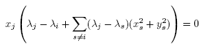
and

If  was a repeated eigenvalue, say
  then letting
 it follows that the equations above hold for any choice of
 so the critical points of f are not isolated and therefore it is not a Morse function; the "only if" part of the proposition is thus proved.
Conversely, suppose . Setting j = 1 in the previous two equations and using the fact that the
  are in increasing order, it follows that x
i = y
i = 0. Inductively one gets
are in increasing order, it follows that x
i = y
i = 0. Inductively one gets Similarly starting with j = n +1 and inducting backwards one concludes
  for each j ≠ i. Hence the unique critical point of f in Ui is the point [0,..., 1,..., 0], where the 1 is in the ith position. So there are n +1 critical points in total, and their corresponding values are distinct (they are the
 ). To check non-degeneracy, it follows easily from the previous computation that the determinant of the Hessian at [0,..., 1,..., 0] in the ith inhomogeneous coordinates is just

which is non-zero because the are distinct. 
The previous analysis now allows us to prove the second and final theorem.
Proof of Theorem 1.5. As in the proof of Theorem 1.4, we must verify conditions (C1) and (C2) of Lemma 2.1. This time the generic function in the Ai-eigenspace has the form of f in Proposition 4.1, with the condition tr(A) = 0,  Write
Write  writing

one sees that the dimension in this case is n(n + 2) and the following set is a basis:

The coefficients of f for this basis are the bij and the cij for i < j, and the bii for i < n +1 (since cii = 0). Noticing that the bij, cij and the aij are bijectively and bicontinuously related, we may diagonalize A =  and finish verifying the same condition (C1) with the same argument as that of Theorem 1.4. Now, for condition (C2) , the argument in Theorem 1.4 (again appealing to Lemma 2.1) gives the estimate

for the projection of f onto the jth eigenspace, and the result follows in the same way since  = 4j(n + j) and (
 ) are polynomials (of degrees 2 and 2n +1)in j.


