


 Inglês (pdf)
 Artigo em XML
 Referências do artigo
 Enviar este artigo por email
 Citado por SciELO
  Citado por Google
  Similares em
SciELO
Similares em
SciELO  Similares em Google
 Permalink
1. Introduction
Structural optimization is a relevant research topic in civil engineering, allowing the structural design process to be formulated as a mathematical programming problem that can be solved by applying optimization algorithms. With its use, better performance and efficiency of the structures [1], savings in the use of resources (e.g., materials) [2], and faster and automatic implementation of the design (in comparison with the traditional design process) can be obtained in reasonable computational times [3].
Trusses are widely used in civil engineering (e.g., roofs, sports stadiums, bridges, and power transmission towers) [4,5]; they are versatile, light, simple installation, and adaptable to diverse geometrical configurations [6-8]. Recent single objective structural optimization studies (power transmission towers) report material savings ranging from 6% to 12% [6,9,10] less than the initial design. Many structural optimization problems of trusses have been solved based on a single objective function, usually structural weight [11,12]. However, in practical situations, the designer must identify several objective functions (the most convenient) to measure economy, strength, serviceability and other factors affecting the structure's performance [1]. In the design of a structure, the goal is generally to obtain minimum cost and higher safety or minimum weight and higher stiffness. These objectives are opposed and generate conflict since improving one implies damaging the other. Multiobjective optimization techniques based on metaheuristic algorithms are a suitable tool for the solution of this type of problem [13,14] and are extensively employed in this work.
In this context, three types of optimization can be applied to trusses: size, shape and discrete topology. Size optimization finds the value of the cross-sectional areas; shape optimization searches the nodal positions.; discrete topology optimization searches the connectivity pattern of the nodes for a defined ground structure (a structure that contains all possible geometrical configurations), allowing the presence or removal of elements and nodes. Topology optimization is the most general problem since it deals with all the possible configurations, instead of one in particular (for size and shape optimization). Its application in real scale structures can result in greater material savings by potentially searching for the best topology [12].
Many truss topology optimization studies reported are single objective function (mainly minimizing weight) small-scale benchmark problems (SOSS problems) and are based on applying metaheuristic algorithms as optimization methods. In order to solve SOSS problems, Hybrid Genetic Programming (HGP) [11], Heat Transfer Search (HTS) [12], Firefly Algorithm (FA) [15], Search Group Algorithm (SGA) [16] and Passing Vehicle Search Simulated Annealing (PVS-SA) [17] have been used. For multiobjective topology optimization small scale problems (MOSS problems), the studies mainly consider the simultaneous minimization of the structural weight and the maximum displacement of the nodes as objective functions: Multiobjective Genetic Algorithm (MOGA) [18], Multiobjective Adaptive Symbiotic Organisms Search (MOASOS) [19] and Multiobjective Uniform Genetic Programming (MUGP) [20].
On the other hand, large-scale (hundreds of elements [5]) truss topology optimization applications are limited. In [9,21,22], modules (groups of elements with predetermined topologies) are used during the topology optimization process to minimize the weight. In [23], the AMOSA, SPEA and PBIL algorithms were applied to the 3D tower topology optimization problem for multiobjective problems. Additionally, many of the large-scale studies have been addressed with only a size optimization approach and a single objective [5,6,24] and few with multiobjective [25-28].
Truss topology optimization problems have been approached mainly with the ground structure approach (see [15,17]), based on a reduction process where elements and nodes are removed of an initial structure (with several possible initial elements, defined ccording to the potential connections between the nodes that make up the search space) until the best possible solution is found [29]. As the ground structure influences the final topology, the method used to generate it is very important. If a method can generate a well-defined ground structure with only a few nodes (in key positions) and a moderate number of bars, this can help obtain a good topology and decrease the computational cost, which is very significant in large-scale problems [30]. Among the methods used to generate the ground structure are: the classical connectivity level method [29], the macro-element method [31], and the stress trajectories method [30,32].
The general purpose of topology optimization is to find the optimal load paths to the supports (i.e., the best nodes and bar connections) [32]. In this context, the use of optimization strategies based on stress trajectories [30] to generate the ground structure may be helpful since, for equivalent load and support conditions, the trusses obtained with topology optimization coincide (in a discrete way) with the principal stress trajectories of an optimal continuum structure [33]. In [34], they presented the constructive topology optimization method PSL (Principal Stress Lines) based on stress trajectories to locate the material and define the geometry and topology of the structure. In [35], they proposed an approach to optimize lattice-core structures using stress trajectories. In [36], they presented a methodology for 2D and 3D topology optimization of lattice structures using the principal deformation trajectories to define the orientation of structural elements.
Considering the discussion above, this work presents a novel large-scale truss multiobjective topology optimization process and its results when applied to planar trusses. The optimization is implemented in two stages: (1) For a continuum planar design space and boundary conditions known, the ground structure topology is generated using the concept of stress trajectories. (2) Using size optimization, the topology generated in the initial stage is optimized by applying three efficient and popular multiobjective metaheuristic algorithms (in terms of their citations); these are: Non-dominated Sorting Genetic Algorithm II (NSGA-II) [37], Multiobjective Particle Swarm Optimization (MOPSO) [38] and Archived Multiobjective Simulated Annealing (AMOSA) [39]. Applying the idea of selecting the best non-dominated solutions provided by each of the three algorithms, a single Envelope Pareto Front (EVP) is found (making an analogy to the design envelope), achieving a greater convergence and diversity compared to the individual performance of the algorithms. The individual performance of the three optimization algorithms (NSGA-II, MOPSO, AMOSA) was evaluated using the Hypervolume metric [40]. The stress trajectories were calculated with the method proposed by Beyer [41].
The outline of this work is as follows: a detailed explanation of the multiobjective optimization problem is presented in Section 2. In Section 3, the stress trajectories are studied and defined. In Section 4, the proposed multiobjective topology optimization algorithm is introduced and, in Section 5, a large-scale truss design example that proves the proposed algorithm's effectiveness is offered. Finally, in Section 6, the conclusions are presented.
2. Multiobjective optimization and multiobjective metaheuristic algorithms
The optimal solution of a multiobjective problem (MOP) is not a single, but a set of solutions considered equally important and defined as Pareto-optimal solutions. This set of solutions represents the compromise solutions between the different conflicting objectives. The main goal of the resolution of a MOP is to obtain the Pareto optimal set and, consequently, the Pareto front. Using the Pareto front the preferred solution is selected according to the priority of the objective functions, the experience of the decision-maker, and (or) other criteria [42]. A MOP is formulated according to Equation (1) [40].
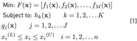
where, F (x) represents the vector of the M objective functions to be optimized. x = (x 1 , X 1 , . . . x n ) is a solution with n design variables. h k (x) and g j (x) are the equality and inequality constraints. x i (L) and x j (U) are the boundary limits of the decision variable x i . In the following, the fundamental concepts in multiobjective optimization are addressed.
2.1 Pareto dominance and Pareto optimality, Pareto optimal set and Pareto front
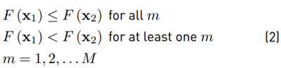
Pareto dominance is used to compare and sort the solution vectors x in a MOP. One vector solution x1 dominates another vector solution x2 (denoted as x1 ≺ x2) if and only if (in the context of a minimization problem) Equation (2) is satisfied [40].
A solution x, is said to be Pareto optimal (not dominated), if and only if there is no other solution X *that dominates it [13]. The Pareto optimal set refers to the values of the decision variables x for the non-dominated solutions (not dominated for any member of the set) in the decision space [40]. Finally, Pareto front is the image of the Pareto optimal set in the objective space [42].
2.2 Goals of a multiobjective optimization problem
Getting the Pareto front is the primary goal of a MOP. A good approximation of the Pareto front must contain a limited number of solutions that meet the following conditions: (i) convergence: be as close as possible to the true Pareto front, and (ii) diversity: find solutions as diverse as possible, i.e., evenly distributed along the non-dominated Pareto front [42]. When the actual Pareto front is unknown, the Hypervolume (HV) metric can be used [40]. The hypervolume measures the volume (in the objective space) covered by the calculated Pareto front solutions, in problems where all objectives are minimized. Its use is recommended using a normalized scale for the objective function values.
2.3 Multiobjective metaheuristics algorithms (MOMAs)
MOMAs are multiobjective optimization techniques oriented towards the direct computation of the Pareto front in a single run, simultaneously optimizing the individual objectives. However, the main disadvantage of these algorithms is the setting of additional parameters related to their functioning and a decrease in the resulting quality in the optimization process when the number of objectives increases. They are beneficial in problems with no information about preferences or priority of objectives [40]. Generally, they have adapted versions of the single-objective metaheuristic algorithms (e.g., Genetic Algorithm (GA), Evolution Strategy (ES), Simulated Annealing (SA), Particle Swarm Optimization (PSO), Ant Colony Optimization (ACO), Harmony Search (HS) among others). These techniques have been established as efficient optimization techniques to solve multiobjective problems. Because of their reliability, free derivative nature and wide use, in this work, the following three multiobjective metaheuristic algorithms were used: Non-dominated Sorting Genetic Algorithm II (NSGA-II) [37], Multiobjective Particle Swarm Optimization (MOPSO) [38] and Archived Multiobjective Simulated Annealing (AMOSA) [39]. The parameters used for each algorithm are presented in Section 5.2.
3. Definition of stress trajectories
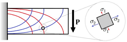
Stress trajectories are tangential lines in the direction defined by the principal stresses at each point of the design domain. For plane stress (σ x , σ y and τ xy ), the principal stresses σ 1 and σ 2 produce two stress trajectories that form an orthogonal network composed of shear-free lines. These trajectories are very useful to understand the load paths (how external loads move through the structure to the supports), provide information related to how the flow of the principal stresses occurs in the plane of analysis, and are related to structural optimization [43,44]. The direction of the principal stresses can be obtained by applying the stress transformation equations at each point of the design domain, given the numerical information of the plane stress state (for a continuous arbitrary design domain, it can be determined using the finite element method). Figure 1 schematically shows the stress trajectories distribution for a cantilever beam with a point load at the free end.
Equation (3) gives the differential equation for a stress trajectory in the xy plane (3):
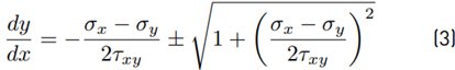
For some special cases, Equation (3) can be solved analytically. However, most stress distributions have complicated shapes requiring numerical methods to approximate the solution [43]. This last option was taken in this work.
4. The proposed multiobjective topology optimization process
The multiobjective topology optimization process presented in this paper applies to planar trusses. It was performed in two stages: An initial stage where, using the stress trajectories, the ground structure's optimized geometry (topology) is generated from a continuum design space with known boundary conditions. In the second stage, applying size optimization, the ground structure generated in the initial stage is optimized to simultaneously minimize weight and strain energy. The multiobjective metaheuristic algorithms NSGA II, MOPSO and AMOSA are used as optimization methods. The general strategy proposed in this paper aims to generate a ground structure with a reduced number of nodes (located at key points) and elements (in the directions defined by the stress trajectories), which is optimized by combining the capabilities of the three MOMAs algorithms (see Section 2.3) to improve the results of convergence and diversity using the EVP concept. The following section presents a detailed description of this process.
4.1 Description of the strategy to generate the ground structure
The strategy to generate the ground structure requires user interaction in some key steps of its generation. It consists of 5 steps, one step implemented in ANSYS® [45] (Step 1) and four steps in MATLAB® [46] (Steps 2 to 5). The steps are shown schematically in Figure 2, and a detailed description of the steps is presented subsequently.
Step 1: Computing the plane stress state
For a continuum design domain, the plane stress state with defined boundary conditions (external loads and supports) is calculated (see Figure 2a).
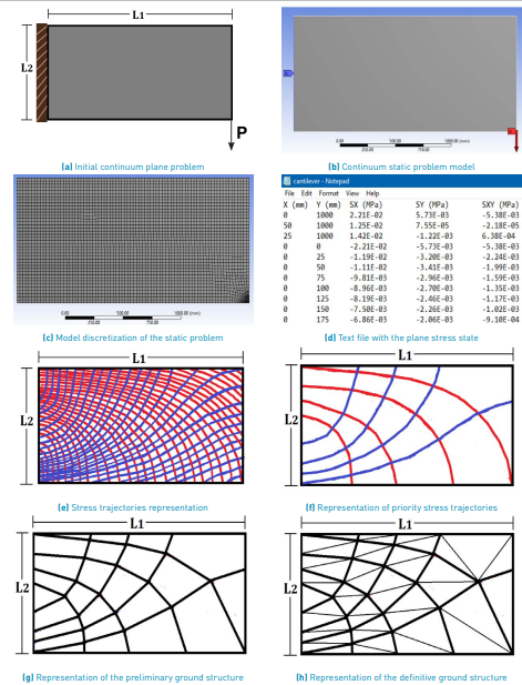
The static problem is solved using ANSYS® considering a homogeneous, isotropic material with elastic properties (see Figure 2b). A text file (.txt) (see Figure 2d) with the numerical information of the plane stress state (σ x , σ y and τ xy ) associated with the design domain discretization in Figure 2c is obtained.
Step 2: Detailed calculation of stress trajectories
Implementing the method developed by Beyer [41], the numerical information of the plane stress state (text file of Figure 2d) is used to interpolate and approximately calculate (using discrete points) the two families of stress trajectories σ1 (red color) and σ2 (blue color), as shown in Figure 2e. The application of the numerical method [41] requires the setting of the following parameters:
Defining an interpolation technique to determine the stress state in an arbitrary point in the continuum design domain, using the discrete information in the text file. The Inverse Distance Weighting method (IDW) [47] was used in this work.
Defining an iteration point (IP), where the computation of the stress trajectories starts. The designer arbitrarily defines its location (within the limits of the design domain); however, it is recommended that this point be located far from the points where the loads and supports are placed, in which the stress trajectories tend to lose their regularity and present sudden changes in their direction because they are singular points (σ x = σy and τ xy = 0) [44].
Step size r, to calculate the discrete points of each stress trajectory. The recommended value for r is L/100, where L is the smallest edge dimension in the design domain [41]. For Figure 2e, the value of L is L 2.
Separation value among stress trajectories a. The user defines an arbitrary value depending on the required resolution.
The total number of calculated stress trajectories depends mainly on problem boundary conditions and the separation value among trajectories a. Initially, a high number of trajectories is required to know how they are distributed in the design domain, so a relatively small value of a is assumed. Moreover, the quality of the results and the computational cost of the numerical method [41]depend on:
Details of the discretization in ANSYS®. More detail implies more data in the text file with the stress state, improving the interpolation quality of the stress trajectories; however, the computational cost can significantly increase, since there is more processing information for the IDW interpolation method.
Separation among trajectories a. A smaller separation value implies an increase in the number of trajectories, a better resolution, and a higher computational cost.
Step size r . A smaller value of r means a better resolution of the trajectories and a higher computational cost.
The processing specifications of the computer.
The problem scale, i.e., the size of the design domain.
In order to reduce the computational cost of the numerical method, the symmetry properties of the structure can be used, and the detail of the numerical model in ANSYS® can be reduced (applying meshing techniques to calculate the representative information for the stress state with the least possible discretization).
At this point, the goal is to obtain a representative number of trajectories with reasonable computational costs, to observe in detail the orientation of the principal stresses in the entire design domain, to identify the priority stress trajectories (the most important of all the calculated trajectories, representing the principal stress paths) used to construct the ground structure.
Step 3: Selection of the priority stress trajectories
The ground structure is generated with the priority stress trajectories, since using all the calculated stress trajectories σ 2 (see Figure 2e) may be impractical, considering that a high number of nodes and elements are generated. Accordingly, a strategy to generate the ground structure using a reduced number of stress trajectories is used. The strategy consists of selecting the priority trajectories, which transmit a higher value of stress or are more expensive (which means higher loads) [32]. The cost concept is directly related to the general objective of topology optimization, which is to determine the optimal material distribution in a design domain, prioritizing areas where the loads are transmitted and the largest stresses occur [30,33]. The sub-steps for selecting the most expensive trajectories are:
Measuring the cost of each trajectory: for each of the stress trajectories σ1 and σ2 in Figure 2e, the average principal stress value of the trajectory is calculated (σ̅1 or σ̅2, respectively). Since each trajectory is a set of discrete points in space along the direction of the principal stress (σ1 or σ2), the cost of the trajectory is the result of computing the average principal stress value of the points that compose it. As a result, the transmission load cost along the trajectory can be approximately measured.
Trajectories classification record: a record is created to classify the trajectories of each family (σ1 and σ2), according to the cost value. The trajectories σ1 are classified in descending order since they are maximum principal stress (or tension) trajectories. Trajectories σ2 are classified in ascending order since they are minimum principal stress (or compression) trajectories.
Identifying the most expensive priority trajectories: for each of the essential nodes (where loads and supports are located), the derived trajectory (σ1 or σ2) that has the highest cost is identified, according to the classification record. Following the consulted literature [32] and preliminary computations performed in this work, the most expensive trajectories are usually derived from the essential nodes. These trajectories must always be present to construct the definitive ground structure.
Identifying additional priority trajectories: to construct the definitive ground structure, it is necessary to include some stress trajectories that are not derived from the essential nodes, to maintain the geometry defined by the stress trajectories. Their assignment can be done in two ways: (1) The user indicates the percentage of the original trajectories in Figure 2e (from each family σ1 and σ2) to include in the final ground structure, following the classification order of the record. (2) arbitrarily, the user defines the additional trajectories to be included, according to the record. Thus, it is possible to get a reduced number of stress trajectories (see Figure 2f), representing the highest cost.
Step 4: Calculation of the preliminary ground structure
The nodes of the preliminary ground structure are located at the points of intersection between the priority stress trajectories and the boundaries of the design domain in Figure 2f. To avoid manufacturing and construction problems (e.g., very short elements), nodes that are very close to each other are adjusted in a single common node. In addition, the designer can manually remove nodes that are not considered necessary. The straight lines among the intersection nodes form a polygonal elements mesh (called macroelements [41]), keeping a geometry that resembles the priority stress trajectories (with a minimum number of trajectories, the aim is to maintain their original shape when they are converted to macroelements), representing the preliminary ground structure, as shown in Figure 2g.
Step 5: Calculation of the definitive ground structure
The preliminary ground structure shown in Figure 2g is used to create additional connections within each polygon with more than three sides to generate a triangular stable ground structure (see Figure 2h). These elements are randomly generated in each polygon. In this way, the definitive ground structure with an optimized geometry (topology) is generated. By applying the strategy proposed in [48], the elements are organized in groups (user-defined value) to reduce the number of variables. The elements are grouped depending on the axial loads obtained in a preliminary analysis, where they are all assigned the same cross-sectional area.
4.2 Mathematical formulation applied to the multiobjective optimization problem
Following the strategy described in Section 4.1, the ground structure (see Figure 2g) is composed of a small number of strategically located nodes in the design domain. These nodes are connected by elements oriented in the directions defined by the stress trajectories (except for the additional connections that stabilize the structure and the initial search space boundaries) and are organized into n groups of variables. Thus, the optimized geometry (topology) of the ground structure is initially known, so the elimination of nodes and elements is not considered during the optimization process, and the mathematical formulation of size optimization is applied as follows:
Finding the value of design variables (cross-sectional areas of the elements) x = (A 1 , A 2 , . . . A n ) that simultaneously minimize the weight (W) and strain energy (E s ) of a planar truss (as shown in Figure 2g), generated with the procedure in Section 4.1. The mathematical formulation is given by Equation (4)
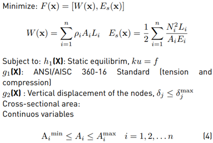
where A i , ρ i , N i , L i and E i represent the design variable area, material density, axial force, length, and elasticity modulus for the i element, respectively. K u and f are the global stiffness matrix, the nodal displacements vector nd the external nodal forces vector over the structure. δ j is the calculated displacement for node j and δ j max is the maximum allowable displacement. A i min and Aj max are the design variable Ai limits in the continuous nterval. ANSI/AISC 360-16 Standard [49] requirements for the design of tension and compression elements (without considering connection design and using the LRFD method) were used in this work and for further detail, the reader could refer to this Standard.
Description of the strategy for handling constraints
The constraint h 1 (X) is satisfied by applying the direct stiffness method (implemented by the authors in MATLAB®). The cross-sectional area constraint is satisfied during the optimization process because the search space limits the design variables. g 1 (X) and g 2 (X) constraints are handled using the constrained tournament technique [40], adapted to multiobjective optimization problems. This technique does not require penalty parameters and can be used especially with population-based optimization algorithms (e.g., NSGA-II).
4.3 Description of the strategy to solve the multiobjective optimization problem
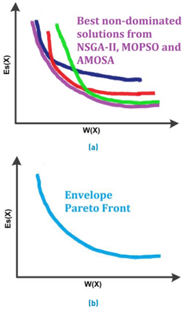
Following the mathematical problem presented in Section 4.2, the ground structure represented in Figure 2h is optimized using the multiobjective metaheuristic algorithms NSGA-II, MOPSO and AMOSA. The best result obtained with each one of the algorithms is a Pareto front with non-dominated solutions distributed along with the two objectives (weight and strain energy), as illustrated in Figure 3.
Applying the idea of combining the NSGA-II, MOPSO and AMOSA Pareto fronts, a single non-dominated Pareto front with the best solutions of the optimization process is calculated (see Figure 4a). In this work, this is called an Envelope Pareto Front-EVP (in analogy to the structural design concept of the envelope), as shown in Figure 4b.
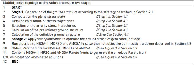
A pseudocode summarizing the proposed multiobjective topology optimization process is presented in Table 1.
5. Numerical example and results
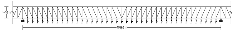
This section shows the validation results of the optimization process presented in Section 4. Its performance is assessed by the solution of a large-scale structure. This structure is a continuous bridge truss (see Figure 5], studied by [50].
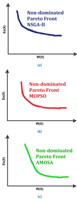
Figure 3 Representation of Pareto fronts for the multiobjective topology optimization problem calculated with NSGA-II (left), MOPSO (center) and AMOSA (right) algorithms
The truss has a span L=200 m and a height h=10 m is assumed (the original study applies shape optimization and a minimum value of h=5 m is established for the upper nodes due to operation and construction limitations). The structure is subject to vertical loads P acting on the lower unsupported nodes with a dead load value DL=-120 kN and live load LL =-80 kN. The material is assumed to be steel (Fy=240 MPa and E=200 GPa). There is a displacement constraint of L/240 in the vertical direction for all nodes. The load combination 1.2DL+1.6LL is considered for designing the structural elements. The displacement constraint is evaluated with the service loads. The problem is solved using continuous variables (as studied initially by [50]) in the interval [500, 60000]mm2. Tubular section elements with a radius of gyration calculated with the expression r=0.4993A0.6777 were assumed.
A personal computer with the following features was used in all tests presented here: Operating system Windows 10, Processor Intel ® Core ™ i5-3230M CPU @2.60GHz and RAM: 8.0 GB.
5.1 Generating the ground structure
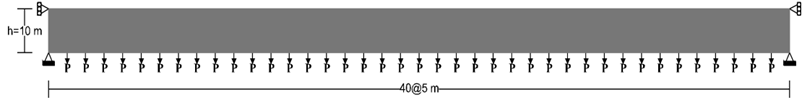
From the initial discrete structure shown in Figure 5 and according to the strategy presented in Section 4.1, the continuum model used to generate the ground structure is shown in Figure 6.
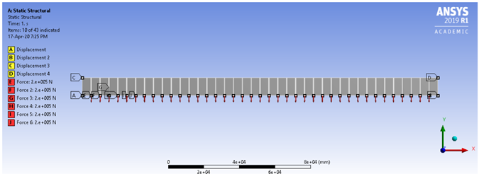
The continuum model in Figure 6 was analyzed in ANSYS® (see Figure 7], to obtain the numerical information on the plane stress state. A 200 mm quadrilateral element discretization mesh was used.
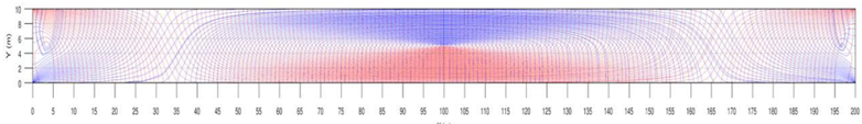
From the stress state numerical information, the stress trajectories σ1 (red) and σ2 (blue) were calculated in MATLAB®, as shown in Figure 8. The parameters used to calibrate the numerical method [41] were: IDW method as stress state interpolation technique, initial iteration point P = (10.0) m, step size r = 100mm and trajectory separation value a=1m.
According to Figure 8, an approximate solution that allows seeing how the distribution of the stress trajectories is in the whole design domain was obtained. The computational time spent on the calculation was 67 hours and 45 minutes. The numerical method may seem expensive; however, considering the scale of the problem, the calibration parameters and the features of the computer used, the calculation time is reasonable. The recommendations described in Section 4.1.2 were implemented to reduce the computational cost significantly.
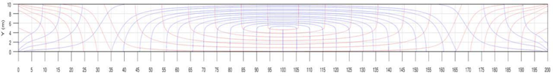
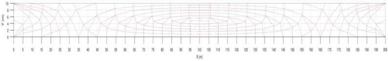
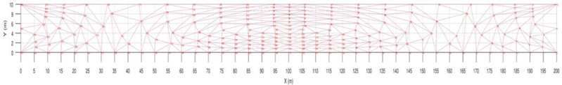
After calculating the stress trajectories in detail, following the steps in Section 4.1.3, Section 4.1.4, and Section 4.1.5, the priority stress trajectories were identified (see Figure 9], the preliminary ground structure (see Figure 10] and the final ground structure [Figure 11] were constructed. The generated ground structure has 240 nodes and 651 elements clustered into 26 design variables (a number defined from the preliminary structural analysis).
The data supporting the results reported in Figure 8 to Figure 11 are available in Zenodo repository: https://doi.org/10.5281/zenodo.4304951
5.2. Optimization results of the ground structure
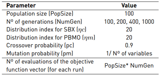
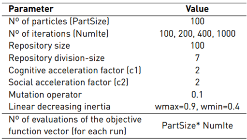
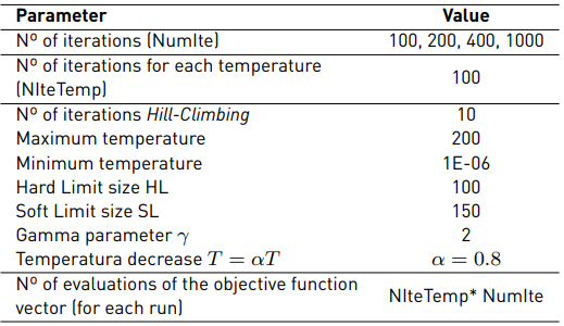
The ground structure in Figure 11 was optimized according to the strategy described in Section 4.3. The parameters used to implement each metaheuristic algorithm are shown in Tables 2, 3 and 4, and were adapted from [37-39]. Each algorithm was run five times using these parameters.
Next, in Figure 12, graphic performance results (Pareto fronts) for NSGA-II, MOPSO and AMOSA are presented. The simultaneous representation of the Pareto fronts for the five runs (for each algorithm) is included, showing their evolution in four control points: 100 iterations in row 1: (a), (b) and (c). 200 iterations in row 2: (d), (e) and (f). 400 iterations in row 3: (g), (h) and (i). 1000 iterations in row 4: (j), (k) and (l).
The quantitative performance results of the NSGA-II, MOPSO and AMOSA algorithms using the HV metric are presented in Figure 13a (using boxplots). The computational cost in seconds is shown in graphically in Figure 13b (using boxplots). The results were calculated for each of the five runs for iteration 1000, where the best solutions were obtained.
According to Figure 12, the best performing algorithm was NSGA-II, followed by AMOSA and MOPSO. The NSGA-II algorithm presents a Pareto front (for each of the five runs) with better convergence and diversity as generations (iterations) advance.
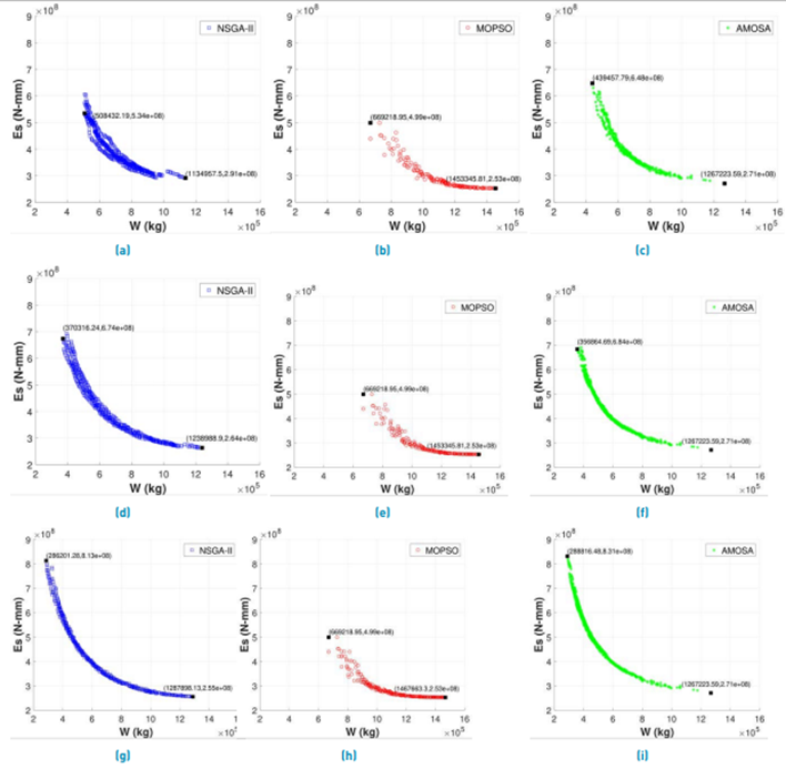
The main variation in results is presented until iteration 400, where solutions are closer to the objective function minimum weight and are distributed over a wider region of the Pareto front, since from generation 400 to 1000, the new solutions are concentrated in the region of minimum strain energy and their generation in the region of minimum weight is more limited. AMOSA presents the main variation of results until iteration 400, in which a set of solutions similar to the NSGA-II Pareto fronts is obtained, and from this iteration, there is a slight variation of results, and the response obtained in iteration 1000 is very similar to iteration 400. Moreover, MOPSO presented convergence and diversity difficulties in this problem (both for continuous and discrete variables), being trapped since the initial iterations in the intermediate region and in the minimum strain energy region of the Pareto front, and it was not possible to obtain solutions close to NSGA-II and AMOSA in the minimum weight region.
Quantitatively, with the results of Figure 13a, (for the iteration 1000), it is shown that they correspond to the graphical results since the best algorithm was NSGA-II, with an HV value closer to 1 (ideal value) and presented little variation between runs (good consistency).
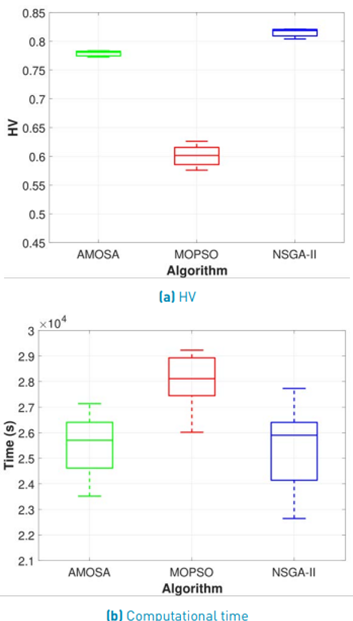
AMOSA presented HV values similar to each other (for each run) and close to NSGA-II. MOPSO presented HV values lower than NSGA-II and AMOSA, and more far from 1. Regarding the computational cost, the time spent by each algorithm per run (see Figure 13b), using the parameters in Table 2, ranged from 21600 s (6 h) to 28800 s (8 h). The mean cost per run for both continuous and discrete variables was 7 h for NSGA-II and AMOSA, and 7 h 50 minutes for MOPSO. The computational costs were relatively high, considering a large number of iterations (1000) and the scale of the problem.
Moreover, Figure 14 shows the convergence of the extreme values (minimum weight and minimum strain energy) of the Pareto front during the 1000 iterations for each of the algorithms (NSGA-II, MOPSO and AMOSA) in each of the five runs.
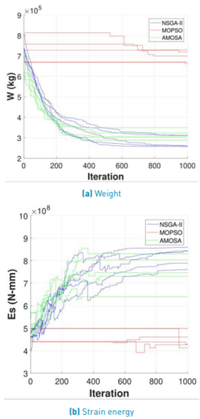
Figure 14 confirms the results shown in Figure 12, where the NSGA-II and AMOSA algorithms tend to stabilize in iteration 400, and MOPSO presents a lower convergence. For the weight objective function (see Figure 14a), the best algorithm was NSGA-II, since compared to AMOSA, from iteration 400, although the convergence rate is lower than in the previous iterations, it continues to find lighter solutions until iteration 1000. MOPSO slowly converges from the initial iterations. The objective function strain energy behavior in Figure 14b is opposed to the weight function since as the iterations advance, its value increases (more strains) as lighter structures are found. Moreover, to validate the strategy for generating the ground structure and its optimization, the minimum weight solutions of the Pareto fronts (see Figure 12] were compared with the optimization results reported in reference [50], as shown in Table 5.
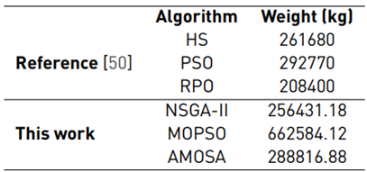
According to Table 5, NSGA-II performed better than HS and PSO. MOPSO did not improve the reference results, considering the convergence problems in this case. AMOSA obtained better results than PSO. Even though none of the three multiobjective algorithms NSGA-II, MOPSO and AMOSA improved the Ranked Particles Optimization (RPO) results, it was possible to obtain results close to those specialized in a single objective function (PSO, HS, RPO). Similarly, these results show that the strategy implemented to generate the ground structure (using the concept of stress trajectories) has a potential for application since the unknown and optimized discrete geometry of a truss can be obtained from a continuous initial space.
Following the strategy described in Section 4.3, Figure 15 shows the calculation results of the envelope Pareto front (EVP). Figure 15a shows the Pareto fronts obtained by the three algorithms (in a single graph) for iteration 1000 (see Figure 12]. From this information, the EVP was calculated, and it contains the best solutions for the optimization problem (see Figure 15b, respectively).
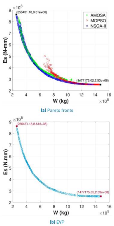
To construct the EVP (see Figure 15b), NSGA-II and AMOSA provided the largest number of non-dominated solutions in the minimum weight region and the Pareto front's intermediate region. MOPSO provided solutions in the minimum strain energy region. Thus, by combining the best solutions of the three algorithms, a broader set of non-dominated solutions can be obtained (compared to the individual results of a single algorithm). Calculating the HV metric of this EVP, a value of HV=0.8252 was obtained, showing a better convergence and diversity than the algorithms' individual results in Figure 13.
Finally, once the EVP with the best non-dominated solutions is found, the designer chooses the most suitable one based on the availability of previous information related to the priority of objectives, environmental and construction criteria, and experience and preferences. If lightweight solutions are required, these are selected from the minimum weight region. If low deformation solutions are required, they are chosen from the minimum strain energy region. When both objectives are equally important, the solutions are selected from the intermediate region of the Pareto front. The data supporting the results reported in Figure 12 to Figure 15 are also available in Zenodo repository: https://doi.org/10.5281/zenodo.4304951
6. Conclusions
The multiobjective topology optimization process presented in this paper is suitable for planar trusses and was developed in two stages. An initial stage in which, for a continuum design space, the optimized topology of the ground structure is generated using the concept of stress trajectories. In the final stage, using size optimization, the ground structure generated in the initial stage is optimized using the NSGA-II, MOPSO and AMOSA multiobjective metaheuristic algorithms to generate a single envelope Pareto front EVP with the best non-dominated solutions.
The strategy to generate the ground structure can be applied to optimization problems that involve a continuum plane design domain. In this process, the designer significantly influences the detailed numerical calculation of the stress trajectories and selects the most important or priority ones (from which the ground structure is generated). Moreover, while the computational cost of the numerical method [41] required to generate the stress trajectories can be high, especially for large-scale structures (see the results in Section 5.1), its use can be beneficial. In this context, a discrete ground structure with an optimized geometry (topology) containing a limited number of nodes and elements located at central sites in the design domain can be generated following the stress trajectories, which provide a guide for the optimal load paths and the locations where the material must be allocated.
The optimization algorithms (NSGA-II, MOPSO and AMOSA) were able to solve the large-scale problem with reasonable computation times, obtaining solutions (Pareto fronts) that satisfy the mathematical formulation. This shows their ability to solve complex optimization problems involving a large number of variables and constraints defined by the design specifications. The obtained solutions were compared with the consulted reference (with only a single objective function, the weight), showing results close to the specialized algorithms in single-objective problems, even when starting (in this study) from an unknown geometry.
Concerning the individual performance of the algorithms in the large-scale problem, both qualitatively (Pareto fronts graphs) and quantitatively (using HV), NSGA-II was the best, followed by AMOSA and MOPSO, for both continuous and discrete variables. NSGA-II obtained a Pareto front that reached the largest convergence and diversity along with the two objectives. AMOSA had similar convergence and diversity as NSGA-II. Moreover, MOPSO had convergence and diversity issues since the initial iterations, providing solutions only in the intermediate region and the region of minimum strain energy. However, by combining the best solutions provided by the three algorithms, a single envelope Pareto front was found, with the largest convergence and diversity (compared to the individual algorithms) and many non-dominated solutions. This suggests that, instead of focusing efforts on finding the most suitable algorithm for a given problem, some of them can be applied simultaneously, exploiting their individual strengths to explore a wider region of the Pareto front along with the two objectives and obtain the best possible optimization results.
Although this work's multiobjective topology optimization process was applied to planar trusses and continuous variables, it is possible to extend its application to three-dimensional trusses with discrete variables by adjusting some of their internal functions (especially the numerical method that calculates stress trajectories). In addition, other types of objective functions and design constraints can be included in the mathematical formulation.
The use of stress trajectories can be extended in additive manufacturing since aesthetically innovative structures (new shapes and connectivity patterns, as in [Figure 8] with good structural performance (elements oriented in the direction defined by the principal stresses) can be obtained using 3D printers and could be very useful in different areas of the industry.

