


 Inglês (pdf)
 Artigo em XML
 Referências do artigo
 Enviar este artigo por email
 Citado por SciELO
  Citado por Google
  Similares em
SciELO
Similares em
SciELO  Similares em Google
 Permalink
1 Introduction
Currently, most of the controllers that are studied and developed are for systems or processes that do not have a delay or have delays so small that they can be neglected, that is, they can be considered within the system time constant [1,2]. For processes whose delays are comparable with these time constants, classical control techniques are not directly applicable. Delays are generally produced by the time of transport of energy or matter within the system. Another origin of the delays are the dynamics of different elements placed throughout the process that, by cascade effect, add up and generate a delay between the input and output that can be considerable [3-5]. From the point of view of control, a single delay can be considered, which is the sum of all [5].
2 Theoretical Formalism
This section describes the basic concepts required in this manuscript, such as delay time, stability, disturbances and finally the structure of the Smith Predictor model, as well as the mathematical apparatus that describes it.
2.1 Delay time (Dead time)
The delay is a phenomenon that passes through the temporary displacement that can appear between two or more control variables and this can be generated, for example, by the time needed to transport mass, energy or information. The dead time or delay can also be due to the sum of all the small delays that the measuring elements present in the system can add [6,7]. Sometimes the dead time can be solved by relocating the measuring elements or using faster response devices, other times it becomes a permanent problem, which makes it necessary to resort to the execution of a compensator [8]. Downtime results in an increase in system phase delay, a decrease in phase gain and therefore a limitation in controller gains and the closed loop response speed [9,10].
2.2 Stability
Stability is the most important specification of a system, because we cannot design an unstable system for a specific requirement of transient response or stable state error. The system is stable if all natural frequencies are in the left complex semiplane. Dead times or delays present in a system reduce the phase margin which implies that the system may become oscillatory and unstable [11 - 16].
2.3 Disturbances
A disturbance is a signal that tends to negatively affect the value of a system's output. If the disturbance is generated within the system, it is called internal, while an external disturbance is generated outside the system and is considered as an input. In a control system, disturbances may be due to external factors due to changes in environmental variables such as temperature, humidity, noise, etc. When the real plant exhibits non-modeled dynamic behaviors and / or is subject to the effect of measurable and non-measurable external disturbances, the effectiveness of the Smith Predictor decreases [12-14].
2.4 Smith Predictor
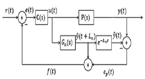
The structure of the Smith predictor (SP) is given by the following internal model representation. Next, a deduction of the closed-loop transfer function for the Smith predictor is presented graphically and analytically (Figure 1 to Figure 4) and analytically (Equation(1) to Equation (8) )[15]. It is then desired to obtain an equivalent controller for the system that contains the loop generated by the prediction system. Initially from the diagram of the Figure (2a) we obtain the transfer function C(s) to the blocks in parallel [5] (Equation (1)). A and from the diagram corresponding to the Figure (2b) we obtain the transfer function C eqs (s) to the blocks in parallel [5] ( Equation(2)).


The closed loop is obtained with the equivalent controller for the system (Figure 3): The closed loop transfer function for the system with the Smith predictor is given by the Equation (3):


Replacing the equivalent controller obtained in the closed loop transfer function must Equation (4):

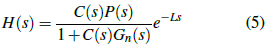
The delay transfer function would be represented as follows, Equation (5):
To model the disturbances on the system, it can be considered that they act as an input, therefore, the expression that relates these disturbances with the output of the system is (Equation (6)):

Thetermal system is presented in the Figure (4), where T is the entering liquid temperature in Celsius degrees °C, T is the temperature of the liquid leaving, G is the liquid consumption in units of Kg/s, M is the mass of the liquid in the tank, in Kg,C p is the specific heat Kcal/Kg°C, R is the thermal resistance °CsKcal, C is the thermal capacity Kcal/°C and q is the heat flow in Kcal/s.

Considering that the temperature of the fluid entering the system remains constant, we can say that the function that determines the outlet temperature corresponding to the thermal system is the following:


For the study of the system, the following values will be taken in the constants M = 10Kg, CP = 1Kcal/Kg°C, G = 1Kg/s, T(s) = Qi/(10s + 1).
3 Results
Initially we present the block diagram for the thermal system (Figure 5) and the corresponding response with and without delay Figure (6), in order to examine its behavior. In the previous figure, you can see, according to the blue graph, the instability that the system presents when inducing a delay. The green graph shows the control of the system when there is no delay and the red one is the reference. Now the SP structure is introduced and its behavior is displayed. The Figure 8 allows visualizing the behavior of the system when the Smith predictor structure is applied, said behavior is the same as that of the system immediately, but displaced the dead time, which occurs when you have an exact prediction of the plant and the time delay. Now we proceed to analyze the response to disturbances which are considered as one of the limitations presented by the Smith predictor.


4 Conclusions
Smith's predictor is a very good prediction technique when working on systems that have very large delays that can affect the response to the point of making the process unstable, its effectiveness lies in a good estimate of the plant and the delay. Based on the results obtained, it is observed that the set-up time that is achieved in the system with delay by applying Smith Predictor is much less than when adjusting a classic controller for the same system. The settling time achieved with a Smith Predictor is the sum of the system response immediately and the value of the delay. The big problem that occurs when disturbances appear within the control structure, because the disturbance is affected by the dead time, which is added to the time it, takes to dissipate it.

