


 Inglês (pdf)
 Artigo em XML
 Referências do artigo
 Enviar este artigo por email
 Citado por SciELO
  Citado por Google
  Similares em
SciELO
Similares em
SciELO  Similares em Google
 Permalink
Nitrogen (N) is a primary element for the development of plants (Aldea et al., 2006); it is the largest component of chlorophyll, amino acids and proteins that are directly related to leaf greenness (León-Sánchez et al., 2016; Valverde et al., 2021) and plant growth (Malavolta, 2006). Deficiencies associated with N influence leaf size reduction, also, chlorosis occurs due to the inability to synthesize chlorophyll, which generates yellowing in young leaves, and therefore, a decrease in growth (accumulation of biomass) which, in severe cases, can induce physiological plant stress (Alchanatis et al., 2005; Berntsen et al., 2006). Studies developed by Djumaeva et al. (2012) mention that N is a fundamental nutrient for tree productivity, thus, it should be considered in the evaluation of the soil at the time of establishing a plantation, as well as in fertilization programs.
Given the importance of N in developing productive forest crops, it is necessary to implement nutrient evaluation methodologies. There are two groups of tests, destructive and nondestructive, applied to leaf cover (Wang et al., 2014). The destructive test consists of collecting leaves and, through elemental analysis developed in the laboratory, the leaf nitrogen content is determined (LNC), which is an accurate system, but it is a time consuming and expensive process and can cause damage to the plant by reducing the foliar area (Silla et al., 2010; Rotbart et al., 2013).
Alternatively, nondestructive methods are based on the reflectance spectrum of the leaf, which is related to the concentration of N (Dana and Ivo, 2008); among the most common methods, measurement with multispectral sensors (Weber et al., 2006), hyperspectral sensors (Taoet al., 2014), chlorophyll concentration sensors (Chang and Robison, 2003) and commercial photographic cameras (Nieto et al., 2017). The last two are the most widely implemented due to their economical accessibility and rapid and nondestructive evaluation of the plant (Djumaeva et al., 2012; Tao et al., 2014). The SPAD meter (Minolta Camera Co.) is an instrument that allows to measure the chlorophyll concentration and indirectly the N concentration, using a 6 mm2 optical sensor that is fast, nondestructive and straightforward to use, but with limitations in terms of leaf sampling (it must be measured several times) demanding equations of correction that allow doing the real determination of nitrogen concentration (Limantara et al., 2015).
The implementation of photographic cameras can measure spectral information in the spectral bands of the visible spectrum (Ali et al., 2013; Wang et al., 2014). Currently on the market, there are cameras with high resolution (higher than 10 megapixels) with sensors capable of collecting a large amount of crop information (Kipp et al., 2014). Aspects such as canopy structure, leaf area, leaf orientation and biomass accumulation can be easily collected with a color image (Nettoet al., 2002) and processed by software such as R, MATLAB® or Image J (Riccardiet al., 2014). Previous studies on agricultural and shrub species have shown that it is possible to develop N prediction models by extracting color information from leaves by combining photography and greenness extraction in RGB and CIEL*a*b* formats (Conesaet al., 2019).
Studies developed by Hu et al. (2010) allowed the creation of the Triangular Greening Index (TGI), which permits the nitrogen potential to be projected from the red, green and blue bands available in a digital photograph with high sensitivity. Pagola et al. (2009) developed a set of color equations from photographic greenness through the CIEL*a*b* system with shrub species, being the b* parameter, the factor related to N. In all these cases, the luminosity and shooting conditions are relevant, which can generate variations in the green color and thus, in the projections of N (Riccardi et al., 2014).
In the case of forest species, the study of N relationship models with indirect methods is very limited. Coste et al. (2010), with SPAD values, allowing the creation of linear and exponential projection equations of N with ratios greater then 0.80. On the other hand, Barrantes et al. (2018) with tree forest species developed a SPAD index of prediction of N with an indirect method, which allowed to determine prediction ranges from color. In the specific case of the CIEL*a*b* color values relationship with leaf N concentrations, no studies were found for tree species, being a significant information gap. In this context, this study aimed to estimate the leaf nitrogen content from nondestructive methods in Eucalyptus tereticornis and Eucalyptus saligna plantations.
MATERIALS AND METHODS
Experimental site
The study was carried out in a plantation of E. tereticornis and E. saligna located in Cartago, Costa Rica (9°50'57.91'N; 83°54'37.27' W) at an altitude of 1,392 m.The average annual temperature of the site is 24 °C and the annual rainfall is 2,100 mm, distributed over seven months of rain (IMN, 2020).The site presented a flat topography, with a slope of less than 10°, with a clay loam soil, with a pH 5.2, 0.93 g kg-1 of nitrogen content and 0.56 g kg-1 of potassium in the first 15 cm of the soil. The climate of the site was classified according to Köppen-Geiger as a subtropical high mountain oceanic climate (Köppen, 1990).
The plantation was 26 months old, with a sowing spacing of 1.0x1.0 m (10000 tree ha-1). the crop was characterized by having minimal silvicultural management due to its objective for the generation of biomass for energy purposes. A total of 30 individuals per species were selected (20 trees were used for model generation and 10 trees were used for validation, they were not mixed to generate the models) with a homogeneous diameter and leaf area index (Table 1). Three groups were randomized to apply nitrogen treatments 120 kg N ha-1 (N1) and 240 kg N ha-1 N2 and a control treatment (no nitrogen was applied). The application was performed in May 2020, when the rainy season started in the study area. For the research, the evaluations were developed for four months after the application of the nitrogen treatments (the application of the different doses of nitrogen was developed only to guarantee a wide range of nitrogen concentrations in the leaves, which facilitated the development of equations).

Nondestructive sampling of N
According to Valverde and Arias (2018), for each individual, five leaves were selected from the middle part of the canopy, as these are not very old or immature leaves, and are not affected by pathogens or deformities. The selected leaves were evaluated with three nondestructive methods: (i) chlorophyll meter (SPAD), (ii) indirect measurement of color with a photographic camera and (iii) direct measurement with a colorimeter.
The relative chlorophyll content value was made using a SPAD-502 (Konica Minolta®) that has an effective area of evaluation of 6 mm2. For each leaf analyzed, three measurements were taken to generate a mean value; the measurement points were located at the ends and at the midpoint of each leaf according to Valverde and Arias (2018).
Color measurement was carried out by analysis of photographs. Therefore, a Sony camera model Alpha 7 ILCE7K/B was implemented, with a photography dimension of 4000×6000 pixels (24 megapixels resolution) with an interchangeable lens of FE 3.5-5.6 / 28-70. It was implemented with an aperture of f/5.6, ISO 300, with a white balance of 4900k, with automatic posture, and flashed off. The camera was placed on a tripod at 40 cm above the samples, which were placed on a matte black background. The luminosity of the site was 1000 lux and it was photographed after the nitrogen potential Subsequently, the images were processed by means of the Adobe Photoshop CC2020 software, the eyedropper tool was implemented, and a sample of 25 individual points of the leaf was analyzed to determine an average value of the color. The generated color values were handled by the RGB color space (R=Red, G=Green, and B=Blue), with values between 0 to 255.
Direct color measurement was performed with a standardized CIE chromatography NIX Pro spectrophotometer. The color was determined in the 400 to 700 nm range with a 10 mm diameter measurement port. For the reflection of the specular component (SCI mode) was included an angle of 10°, which is typical for the surface of leaves (D65/10); and with a D65 (corresponding to daylight at 6500 K). Selected color space was CIEL*a*b*, which generated three parameters to explain the color that consisted of L* (luminosity) that ranges from 0 to 100, where 0 is black and 100 is white; a* (color trend from red to green), positive values tend to red and negative values to green and b* (color trend from yellow to blue), positive values tend to yellow and negative values to blue.
Destructive sampling of N
The same leaves that were used in the nondestructive analysis were used for destructive sampling. Each leaf was dried at 60 °C for 72 h according to Valverde et al. (2017). Subsequently, it was grounded until the size of the particles was 225 to 250 µm. The material was stored for 72 h in an air-conditioned area (22 °C and 50% relative humidity). The moisture content of the material was 12%, then 0.5 mg of this material was analyzed in an elemental analyzer model Vario Micro Cube to estimate the LNC.
Statistical analysis
First, the Anderson-Darling test (normality test) and the Breush-Pagan test (homoscedasticity test of the variance) were performed on each database obtained from the leaves to determine that there was a parametric behavior in the data; afterward, a descriptive statistical analysis was carried out. The characterization of the different variables was analyzed. To determine the relationships between the LNC and the values of the color spaces under study and SPAD values, simple relationships were performed, in which each color index and SPAD were placed on the X-axis and LNC on the Y-axis, later analysis of Pearson's correlation where the color spaces, SPAD and LNC were correlated in order to eliminate the indices that showed lower correlations. Then multivariate linear regression (selected by previous studies of Baresel et al., 2017) was performed under the model Y=a+b1x1+b2x2+…+bnxn, in which LNC was the dependent variable and the CIEL*a*b* color coordinates, RGB and SPAD measurements were the independent ones, therefore, the regression coefficient was estimated with least squares; For comparison of models, the coefficient of determination, the model error, Akaike Information Criterion (AIC) and Bayesian Information Criterion (BIC) were implemented. Finally, the best color prediction equation was selected for each color and SPAD model was validated according to Valverde and Arias (2020a), the random cross-validation method was used. All the analyzes were developed through the R software version 3.6.2 (R Core Development Team 2020), with a significance of 0.05.
RESULTS AND DISCUSSION
LNC and CIEL*a*b* color space relationship
Figure 1 shows the different relationships between LNC and L*a*b* color space in the two tree species; similar behaviors were determined (All data met the assumptions of normality and homoscedasticity). The LNC values ranged from 0.8 to 2.4%. The luminosity (L*) ranged between 20 and 60 considering a medium to low luminosity (color trend in low light), a* values were negative and ranged from -20 to 0, it can be considered a greenish color trend. On the other hand, b* values obtained tended to yellow colorations, since they ranged from 0 to 60.

Figure 1 Relationship between color by L*a*b* format with leaf nitrogen content (LNC) of plants of E. tereticornis (A, C, E) and E. saligna (B, D, F).
A relationship between LNC and luminosity (L*) was determined as the L* value increased, the percentage of LNC tended to decrease (Figure 1a and 1b), showing a coefficient of determination that ranged from 0.705 to 0.743 considered as significant. Regarding the color a* parameter (Figure 1c and 1d), a clear trend was not found, since a flat behavior was exhibited in E. tereticornis and moderately increasing in E. saligna, but with coefficients of determination lower than 0.13, which may be considered as a poor relationship. Finally, the increase of b* parameter generated decreases in the LNC values (Figure 1e and 1f), being a significant relationship with coefficients of determination higher than 0.722.
The results obtained were similar to those presented by Barrantes et al. (2018) with shrub and tree species for industrial purposes. The a* parameter is not very functional for the development of LNC estimates, because it is a variable of low sensitivity; the greenness of this variable showed low variability compared to the L* or b* parameter. This is because nitrogen losses in the plant tend to generate yellowing, which in the CIEL*a*b* color model, would be perceived by b*, which showed strong correlation with LNC. At high LNC concentrations, yellowing is scarce and increases as LNC decreases, an aspect that Hu et al. (2010) mentioned as a common behavior because low levels of nitrogen generate foliar discoloration due to a lower concentration of chlorophyll and the presence of amino acids and proteins, aspects that Conesa et al. (2019) highlight as indicators of the discoloration process. Therefore, the b* parameter is the best colorimetric indicator to denote the concentration of LNC (Nieto et al., 2017).
In luminosity, the relationship with LNC is due to two reasons as was mentioned by Wang et al. (2014) and Nieto et al. (2017): i) It is a color correction index, in very high or low luminosities, it tends to generate errors in the estimation of the LNC; therefore, it is common to have values close to 50 for a correct color determination and to relate it to LNC. Very high or low values of L* induce variations in the green tone of the plant, which generates under or overestimation of the a* and b* indices. ii) It is a parameter that shows a relationship with the concentrations of chlorophyll in the leaf. High concentrations of chlorophyll, which is an indirect indicator of LNC, tend to have a dark leaf color and low luminosity, it is in leaves with chlorosis in which the luminosity is increased due to low concentrations of chlorophyll.
LNC and RGB color space relationship
Regarding the RGB color space (Figure 2) (All data met the assumptions of normality and homoscedasticity), it was determined that the R (Red) index varied between 40 and 140, while the G (Green) index ranged between 60 and 150 and the B (Blue) index was found within the range from 0 to 80. Relationships between the RGB and LNC color space were determined using the R index (Figure 2a and 2b), a decreasing trend of the LNC as the value of R increased. This behavior was the same in both studied species and with a significant relationship, obtaining a coefficient of determination ranged from 0.736 to 0.746. Regarding the G index (Figure 2c and 2d), a negative behavior was presented. As G value increased, the LNC decreased, presenting a coefficient of determination higher than 0.70 in both species. On the other hand, the behavior varied among species regarding the B index (Figure 2e and 2f). For E. tereticornis (Figure 2e), a slightly positive trend was determined, which as B increased, the LNC increased, with a moderate coefficient of determination of 0.56. In contrast, with E. saligna there was no clear pattern of behavior, and it presented a poor coefficient of determination of 0.09.

Figure 2 Relationship between color by RGB format and leaf nitrogen content (LNC) of E. tereticornis (A, C, E) and E. saligna (B, D, F).
The relationship between LNC, R and G indices were similar to the results obtained by Aliet al. (2013) with agronomic species; the leaves with the highest nitrogen content presented a dark greenish, which increases in the R and G indices, whereas the B index remains with a scarce variation due to the low sensitivity to changes in green. In colorimetric prediction models, Jannoura et al. (2015) and Baresel et al. (2017) mention that R and G layers are very susceptible to leaf color change, as slight variations of both indices can generate significant visual variations of the green color. B Index is not very sensitive and is generally constant in the different shades of green, limiting its use in equations.
LNC and SPAD relationship
Regarding the SPAD evaluation, the values ranged from 10 to 65, finding a direct proportional relationship in both species (Figure 3); as the SPAD value increased, the LNC also increased, with a high ratio the estimated coefficients of determination (0.720). These results are similar to those presented by Coste et al. (2010) with tree species, finding a positive linear relationship. The reason is that the SPAD equipment is developed to measure chlorophyll at red wavelengths (640 to 650 nm) and near-infrared (920-930 nm), points where is possible to find chlorophyll exposure, which is directly related to LNC. Pinkard et al. (2006) reported that nitrogen measurements with instrument are accurate due to the linear relationship with nitrogen; however, they found limitations because in the first stages of stress in the plant, they could not accurately identify changes in nitrogen concentration. It requires moderate periods of stress to identify the variation, since it is a method that requires the development of regression equations to link the indicator with nitrogen directly.

Correlation between LNC, color indices and SPAD
Correlations between LNC, the two-color models used and SPAD measurement showed the same behavior in both study species (Table 2). A strong correlation between LNC and SPAD was determined, being positive and with values higher than 0.850. On the other hand, with the CIEL*a*b* model, the correlations of the L* and b* were high and negative with a value higher than 0.840, whereas with the a* index, no significant correlation was found with values lower than 0.350. Moreover, in the RGB model, R and G indices have a negative correlation with significant LNC with values higher than 0.830. In contrast, the B index varies with the species; for E. tereticornis a strong and negative relationship was found (value of -0.720), while for E. saligna no relationship was found, being an irrelevant indicator.
Table 2 Coefficients of correlation between the LNC values, SPAD measurements and color indices of the CIEL * a * b * and RGB models in leaves of E. tereticornis and E. saligna.
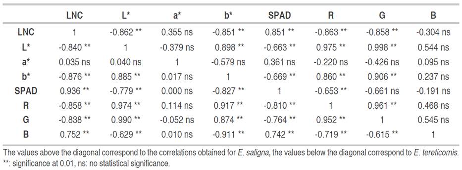
Using CIEL*a*b* space, the L* and b* indices showed a high correlation with LNC, similar to the result presented by Pinkard et al. (2006), Wang et al. (2014) and Nieto et al. (2017) with shrub and tree species, where the relationship of both variables is due to the sensitivity of perception of yellowing, something that the a* index is not able to predict, and which generated its low correlation. Ali et al. (2013) highlighted the b* parameter as the optimal rate of LNC change in the short-term due to its high sensitivity in leaves and easy measurement. By contrast, with the RGB space, the R and G indices showed a high relationship due to the perceived bands of both indices. G is 520- 600 nm, while R is 630 nm, which allows seeing changes in the leaf greenness generated by changes in chlorophyll and nitrogen concentration. Finally, the SPAD is a device that has the functional capability to develop relationships with the LNC, as it was developed to measure chlorophyll in the visible and infrared field.
Equations to estimate LNC from color indices and SPAD
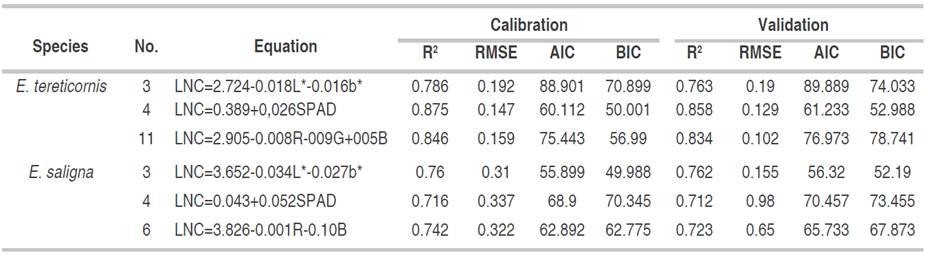
The prediction equations of the LNC from the color indices and SPAD measurements are presented in Table 3. For E tereticornis in CIEL*a* b* model, the combination of the L* and b* indices was determined, generating an equation with a higher coefficient of determination (0.786) and a lower error of 0.198 on developing individual models with each index, it means, CIEL*a*b* color model is the best option to estimate the LNC. In addition, a model with a high coefficient of determination of 0.875 and a deficient error of just 0.147 was generated from SPAD measurement, showing the effectiveness of this methodology to estimate LNC in the studied species. Also, RGB color model was another suitable combination to predict LNC. This combination presented a significantly higher coefficient of determination and a notably lower error than the equations with each index alone or their combinations.
Table 3 LNC estimation equations from CIEL*a* b* and RGB model color indices and SPAD measurements for E. tereticornis and E. saligna plants.

For E. saligna species (Table 3), through CIEL*a*b* model, L* and b* indices in the same equation presented the highest coefficient of determination and the lowest error, AIC and BIC, being the optimal evaluation model. At the same time, an equation with a strong coefficient of determination of 0.716 and a moderate error of 0.337 was determined using SPAD measurements, (AIC and BIC), which showed the potential of SPAD in forest species to predict LNC. Finally, with RGB color model, the RG indices presented the best LNC prediction model, with the highest coefficient of determination (0.742) and the lowest model error (0.322), AIC and BIC, being the RGB color model the best option.
The selection of equations with the indices L* and b* were similar to those selected by Pagolaet al.(2009); the accuracy of the prediction of the appearance of LNC is due to the precision of both color indices in predicting the color change of leaves by nitrogen. In the case of SPAD, Coste et al. (2010) showed similar equations due to the ease of the equipment to estimate LNC, making it a good choice for forest species. In the RGB case, the behavior was different from that reported by Baresel et al. (2017), and who determined that the equations with R and G were sufficient to estimate changes in LNC. In the case of the study, B index had a significant relationship with the LNC appearance due to the characteristics of the species.
Validation of the best LNC estimation equations
The validation of the studied models (Table 4) showed the same behavior for both species. The coefficient of determination and the R2 of the error tended to decrease between 10 and 15% in all equations, finding the best result for E. tereticornis. LNC estimation method was performed with SPAD, as it showed the highest coefficient of determination and the lowest error, AIC and BIC, followed by RGB color model and the lowest accuracy, represented by CIEL*a*b* model. For E. saligna, the B index showed the best statistical values, being the best option for estimating LNC, followed by SPAD and finally the equation of the L* and b* indices.
Advantages and disadvantages of the proposed methodology
The nondestructive methodology implemented showed acceptable estimation values compared to destructive methods or high-cost instrumentation developed for N estimation. Ali et al. (2013) mentioned that the development of nondestructive measurements that estimate N values y are fundamental for intensive crop sampling with the advantage of reducing the cost of sampling, immediate data for making quick decisions, no impact on the crop and short time to generate information.
Nevertheless, the limitations of the photographic technique or SPAD must be considered, such as the dependence on climatic conditions (Baresel et al., 2017), the need for equipment calibration (Ali et al. (2017) and the dependence of the leaf color on the appearance of the plant, for instance, the competition for space, water stress, the availability of light and phytosanitary status, so the selection of sampling plants must be essential in the study and environmental conditions must be controlled (Chang and Robinson, 2003). If the cultivation conditions are controlled and the protocol is clearly managed, equations with significant precision can be obtained, as mentioned Sun et al. (2018) and Valverde and Arias (2020a) for agronomic and forest species.
The applicability of this system simplifies the nutritional assessment process. Equations can be created by species or group of species (which have characterization studies, and distinguished nutritional patterns. This is essential to be able to develop general equations. In case of not having this information parameterized, the generation of unique models is not recommended). It can avoid the process of sending samples to the laboratory and destructive analysis. With photographs collected in the field that follow a luminosity and image homogeneity protocol, nutritional analyses can be developed. Following the methodology proposed by Valverde et al. (2020b), the next step is the use of cameras and equipment of low-cost and greater accessibility that maintains representativeness, which would reduce the costs of the method and expand its application (it is possible to use smartphone or lower-cost cameras with a resolution greater than 8 megapixels).
CONCLUSIONS
It is possible to estimate LNC from indirect, low-cost, fast methods and without generating significant damage to the study plant. Furthermore, in CIEL*a*b* color space, the L* and b* indices showed a strong negative correlation with LNC, because they are two indicators susceptible to leaf chlorosis. In the case of RGB space, the R and B indices showed the most significant negative relationship with LNC, thus, a photographic image can be used in equations for the estimation of nitrogen with an acceptable precision for both study species. Regarding SPAD, its potential for LNC estimation is confirmed once again with positive linear relationships with nitrogen and a correlation higher than 0.75. Finally, the best model for E. tereticornis was LNC=0.389+0.026SPAD with SPAD equipment, while for E. saligna was LNC=3.826- 0.001R- 0.10B generated with digital photography.
The analysis of tropical tree species used in reforestation programs for commercial purposes should be considered for future research, they should be analyzed with different concentrations of nitrogen and water stress to generate different models to estimate nitrogen with nondestructive methods.
In addition, it is recommended to continue with these types of studies in which lower-cost cameras and analysis software are implemented in order to determine if the accuracy in the equations and models with good fit is still maintained.

