


 Inglês (pdf)
 Artigo em XML
 Referências do artigo
 Enviar este artigo por email
 Citado por SciELO
  Citado por Google
  Similares em
SciELO
Similares em
SciELO  Similares em Google
 Permalink
Introduction
Turbulence is much more complex than laminar flow. According to the Boussinesq eddy viscosity assumption (Boussinesq, 1877), the logarithmic law for velocity profile was solved by using the mixing length method (Prandtl, 1925; Khan et al., 2017; Zawar et al., 2017). Some vertical velocity distribution laws, such as the power law and the exponential law, are based on experimental considerations or semi-empirical theories (Lin et al., 1953; Deissler, 1954; Afzal et al., 2007). Other laws for turbulent velocity profile or concentration profile are based on an indirect turbulence model (Bucci et al., 2008; Nucci and Fiorucci, 2011).
Logarithm law is the most popular one used to express the mean velocity in a cross section of turbulent flow for wind flow, river flow, and lake models. The logarithm law fits velocity and concentration distribution in the position far away from the interface in developed turbulent flow (Wang and Yu, 2007). Some researchers have focused on mean velocity profiles of turbulent wall-bounded flows separately (Poggi et al., 2002; Buschmann and Gad-el-Hak, 2007; Kempe et al., 2007; Buschmann et al., 2009).
Different vertical velocity distribution laws are used to describe stream-wise velocity structure in coastal currents (Soulsby, 1980; Anwar, 1996, 1998; De Serio and Mossa, 2014), in tidal channels (Soulsby and Dyer, 1981), and on the continental shelf (Soulsby, 1983; De Serio and Mossa, 2010).Vertical distribution of suspended sediment concentration (SSC) in rivers, estuaries, and coastal currents have been studied by many researchers through the years (Rouse, 1937; Taylor and Dyer, 1977; Li uet al., 2014).This work derives general formulas to describe the mean velocity and SSC distributions of turbulent shear flow to fit the whole cross section from the bottom boundary to the upper boundary, using a probability density function method.
A brief review of classical methods for velocity profile of shear flow
Consider the laminar shear flow-the steady incompressible developed flow between two interfaces, with one interface moving with velocity U and the other being motionless. The flow can be solved based on 2-dimensional Navier-Stokes equations and expressed as
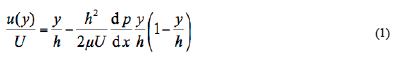
Here h is the distance between two interfaces, μis dynamic viscosity, and d p/ d x is the pressure gradient along the x-direction. The velocity profile of shear flow can be simplified to Eq. (2) when d p/ d x = 0
Logarithm law (Prandtl, 1925), derived by the mixing length method, is the most popular equation used to express the mean velocity in a cross section of turbulent shear flow. The basic logarithm law of mean velocity profile of turbulent shear flow is
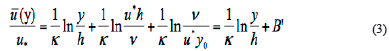
Here, u* is the shear velocity of the fluid and y0 is hydrodynamic roughness length. But Eq. (3) cannot fit select velocity profiles not full profiles because of the assumption that the mixing length is proportional to the distance away from the wall boundary. Many instances and experiments have proven that the mixing length method can successfully predict velocity distributions far away from the interfaces, but it cannot predict velocity distribution near interfaces such as walls, seabed, gas-liquid surfaces, and so on.
As far as we know, turbulent intensity should be dependent on the Reynolds number, which is composed of the characteristic velocity, characteristic length, and kinematic viscosity. Considering the mixing length method carefully, the core assumption is that the eddy viscosity is in direct proportion to the average velocity gradient and the mixing length is in direct proportion to the distance away from the wall. The method does not directly create the relationship between turbulent parameters and average velocity.
Exponential probability density model (EPDM) for mean velocity profile of turbulent shear flow
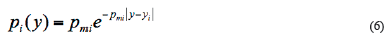
To solve for turbulent flow without closely associated defferent dynamical mechanics, a probability density function method is adopted to describe the pulsating intensity of velocity of fluid particles in this study. The pulsating intensity of every fluid particle in the profile will impact the whole profile. The effect decays at a distance from its original position and obeys a probability density function. Exponential probability density function is often used to describe the decay degree distribution in many physical and chemical problems. In many situations, the exponential probability density function model is an appropriate method to approach the random decay phenomena. The primary expression of the exponential probability density function is
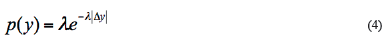
Here, p(y) is the probability density of a fluid particle impacting any position, λ is the damping index, and y is the distance from the particle position yi to the impacting position y, defined by

As shown in Fig. 1, the expression of exponential probability density function p1(y), represents the probability density that the velocity of laminar shear flow at position y1, u1, distributes to any position y due to turbulence. Because the expression satisfies the boundary condition that p1(y1) = pm1 where y = y1 as shown in Fig. 1, λ = pm, such as λ1= pm1, λ2 = pm2, and so on. Hence, the expression pi(y) satisfies
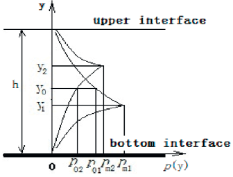
The probability density of u, velocity of any position of y, distributes to y0, a certain position at the profile, is defined as p0 as shown in Fig. 1, such as p01 and p02. We have

average turbulent velocity of a particular position, y0, produced by integrating the product of the local laminar velocity in Eq. (7), which is solved with Navier-Stokes equations, and the exponential probability density function of pulsating intensity at the position, across all fluid particles in the profile, is shown as
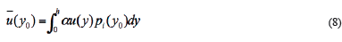
Here α is an adjustment.
Substituting u(y) with Eq. (2) and p0(y) with Eq. (7) in Eq. (8), we get
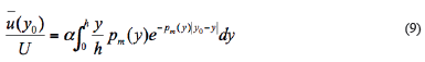
Eq. (9) cannot be analytically and fully solved. To solve Eq. (8), we assume that

Substituting Eq. (2) and Eq. (10) into Eq. (8), the result is
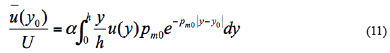
Integrating Eq. (11), the result is
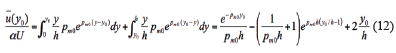
Setting

and substituting y0 with y in Eq.(12), the velocity profile of turbulent shear flow with this method (called PDFM) should be
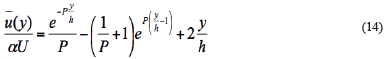
Assume that
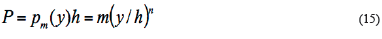
Eq. (14) can be calculated when the adjustable parameters, m and n, are given.
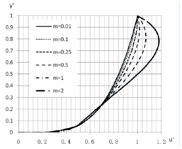
The mean turbulent velocity in Eq. (14) can be calculated by giving different m and n, as well as defining the dimensionless turbulent velocity and dimensionless position as

The calculated results are shown in Fig. 2 and Fig. 3. Fig. 2 reveals that the mean velocity profile changes when the value of m is changed, but the mean velocity changes are weaker in the region near the wall or other interfaces than in the intermediate region while α=1. The dimensionless velocities are almost the same in the region when the value of y+ is between 0 and 0.25, but they change very evidently near the position where y+ is approximately equal to 0.8. Thus, the upper mean velocity will increase along with an increasing value of m. The curve shape fits turbulent velocity profile when the value of m is lower in this case, such as m=0.25, 0.1 and 0.01.
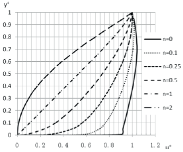
The mean velocity profiles are distinct when the values of n are different, as shown in Fig. 3, while α=1. The main tendency of the profile curves is shifting from the top left to the bottom right in Fig. 3 along with the decreasing value of n. The tendency indicates that the parameter n has a closed relationship with turbulent intensity.
Verification of PDFM in coastal currents
The mean velocity profile model derived in the previous section was applied to fit the investigated profiles to verify the effectiveness of the model. To use Eq. (14) conveniently, the profile formula of PDFM should be transformed as
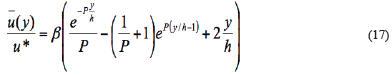
Here β= αU/u*.
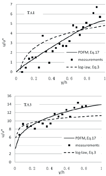
Figure 4 Calculated and measured vertical profiles of the stream-wise velocity of coastal currents at Taranto (Survey data cited in De Serio and Mossa (2014))
De Serio and Mossa (2010, 2014) investigated vertical profiles of the stream-wise velocity of the coastal currents at the Taranto (TA) and Bari (BA) sites in Italy. The comparison between the measurement data, the log law as shown in Eq. (3), and the PDFM as shown in Eq. (17) is plotted in Fig. 4 at Taranto for vertical stream-wise velocity profiles in shallow coastal currents. The calculated results show that the probability density function model (PDFM) more accurately reflects measurement data than the log-law model.
SSC profiles model and its verification in river and estuary
The Rouse equation (Rouse, 1937) was the most popular method used to calculate vertical concentration profiles of suspended load in rivers, lakes, estuarine and coastal currents, as well as on the continental shelf. The Rouse formula was
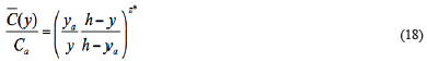
in which ya is the thickness of the sheet-flow layer, Ca is the concentration at ya which equals the bed-load concentration, z*= ω/ku* is the suspension index, and ω is the particle settling velocity. The similar expression of PDFM also can be created by the method below based on the Schmidt diffusion equation (Schmidt, 1925).
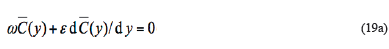
That is
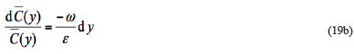
in which ε is the particle diffusion coefficient, set as an assumption of the exponential probability density function
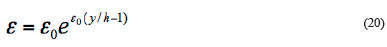
then
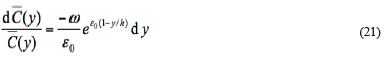
Hence.
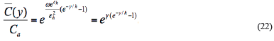
Here γ is the suspension index of this model.
The results of SSC profiles calculated on PDFM of Eq. (22) are shown in Fig. 5.
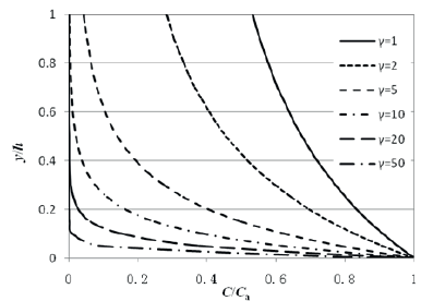
Figure 5 shows that the slope of the profile curves is bigger near the surface than the bottom and the upper slope increases as the lower slop decrease when γ is increasing. The trend means that the particle settlin velocity, particle diffusion coefficient and the water depth velocity influence ' to change the SSC distribution in the vertical cross section.
The SSC is very small when γ=50, so the bed load is the dominan composition when γ≥50. The curves also show that the SSC at surfaces i greater than zero when γ≤2. On the contrary, the SSC at surfaces tends to zer when γ≥2. So, this model provides an approach to avoid the surface limitatioi of Rouse equation.
Zhang et al. (2007) investigated SSC of the Yangtze River in detai and concluded a semi-empirical model of SSC. A comparison of predictin profiles between the PDFM (Eq. 22) and the Rouse equation [Eq. (18)] witl the measurements in the Yangtze River is shown in Fig. 6. As shown in th figure, the PDFM model used for this study more accurately reflects th measurement data than does the Rouse equation.
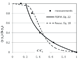
Figure 6 Calculated and measured vertical SSC profile in the Yangtze River (Survey data cited in Zhang et al. (2007))
Liu, Yang, Zhu, et al. (2014) investigated the average SSC profile in the Yangtze Estuary in detail. The survey data is cited here to verify the PDFM model, Eq. (22). The comparison between the Rouse equation, PDFM, and measurements is shown in Fig. 7. The PDFM model of this study is also agreed more closely with the measurement data than does the Rouse equation in the case of the estuarine area.
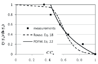
Figure 7 Calculated and measured vertical SSC profile in the Yangtze Estuary (Survey data cited in Liu, et al. (2014))
Discussions
A model for solving velocity and concentration distribution of turbulent flow by using probabilistic methods is put forward in the article (Khan et al., 2017; Sultana et al., 2017). General models for describing the mean velocity and SSC profiles of a whole cross section in turbulent shear flow are derived based on the idea. In fact, the velocity profile formula of laminar shear flow is also the mean velocity profile solution of turbulent flow which ignores the turbulent items in Reynolds equation, thus the pulsating intensity of fluid particles is apparently related to it. On the other hand, the pulsating intensity is also under the control of certain boundary conditions. The exponential probability density function may describe the pulsating intensity of fluid particles of the whole cross section correctly to study mean velocity and concentration distributions. The calculated results of the derived formulas are as diverse as the changing the damping index of exponential probability density function. An innovative approach may be found to solve complex turbulent flow by expanding on this concept.
Conclusions
The PDFM model of this study possesses some advantage in the fields of predicting stream-wise velocity profiles of coastal currents and SSC profiles in river and estuaries as shown in the previous examples. Further research is needed to validate the method through continued studies and carried forward to clarify and optimize the parameters of these models to apply for practical problems. For advanced research, the parameters should be studied meticulously, such as its relationship with dynamic parameters, particularly turbulent characteristic parameters.

