Introduction

Basic research in surface science and interface is highly interdisciplinary, covering the fields of physics, chemistry, biophysics, geographic, atmospheric and environmental sciences, materials science, chemical engineering, among others, specifically the kinetic behavior of the gas - solid interfaces is generally the phenomenon of interest in surface science.

This is the importance of research in the kinetics of surface processes in general. The knowledge of the observable behavior such as sticking coefficient and thermal programmed desorption spectra (TPD) is a particular topic in this area. It is well known that the Arrhenius parameters of the desorption rate constant and the sticking coefficient to be dependent on coverage even in the case of monocrystalline surfaces (^{Heras, et al., 1991}).

The coverage dependence of the activation energy for desorption and sticking coefficient is usually attributed to lateral interactions between adsorbed particles or also explained by interactions via precursor states. Far less consideration has been given to the coverage dependence of the pre-exponential factor for desorption (^{Zhdanov, 1986}).

Materials and methods

Sticking Coefficient. The theory of the adsorption-desorption kinetics on homogenous surfaces is by now well understood. One of the methods used in analyzing the problem is the kinetic lattice gas model (KLGM) applied to the adsorbed layer. This method is based on the approximation of the master equation. In the KLGM, adsorption, desorption and diffusion are introduced as Markovian processes through transition probabilities, which must satisfy the detailed balance principle (^{Kreuzer, 1999}; Luscombre, 1984; ^{Payne, 2002}).

To describe the temporal behavior of the system, a function P(n,t) which gives the probability that a given microscopic configuration n={n ₁, n ₂, ..., n _M} exists at time t is introduced, where M is the total number of adsorption sites on the surface. This probability satisfies a master equation:

Where W(n´;n) is the transition probability that the microstate changes into n´ per unit time. It satisfies the principle of detailed balance (PDB)

P₀ denotes the equilibrium probability.

Usually, the procedure introduced by Glauber is followed, and guesses of an appropriate form for W(n´;n) are made. For a two-dimensional lattice gas with nearest-neighbor interactions where only adsorption and desorption processes are taken into account, the transition probability can be written as

With this, adsorption into site (i,j) occurs if initially n_i,j= 0, with a rate controlled by prospective neighbors if ^{_{Ai ≠}} 0. The Kronecker delta for sites (l,m) ≠ (i,j) excludes multiple transitions.The PDB imposes the next set of restrictions on the coefficients Ai and Di (^{Zhdanov, 1993}; ^{Buendía, 2006}; ^{Kreuzer, 1990}).

^_wa and ^_wd contain the information about the energy exchange with the solid in the adsorption and desorption processes (^{Buendía, et al., 2006}). PDB provides only half the number of relations to fix these unknown coefficients in the transition probabilities. Again, the static (lattice-gas) Hamiltonian cannot completely dictate the kind of kinetics possible in the system. As it is pointed out in Refs. (^{Kreuzer, 1990}, 1997), any functional relation between the Ai and Di coefficients must be postulated ad hoc or calculated from a microscopic Hamiltonian that accounts for coupling of the adsorbate to the lattice or electronic degrees of freedom of the substrate. In addition to the PDB, expressions in parentheses of the equations (6-10) must be greater than zero (^{Buendía, et al. , 2006}) for the dynamic to yield physically correct results.

Whereas in KLGM coverage is defined as

Where the first sum runs over all (M) sites of the lattice. Considering Eq (1) the motion equation for coverage can be written as (^{Kreuzer, 1988},¹⁹⁹⁰,1997; Payne, 1993; ^{Payne, et al., 1993}; Manzi, et al., 2005; ^{Sales, 1987}):

Indicates the average number of occupancy for the second order moment, which evaluates the probability that the site to the right of a site occupied.

Alternatively to the master equation treatment, the rate equation for coverage can be written through of the phenomenological formulation, as a difference between adsorption and desorption terms:

The adsorption term can be specified as a product of the particles flow that reaches the surface from gas phase with pressure P and temperature T, hitting the area ^_as of an adsorption cell, and adsorbing with a probability equal to S (θ,T), i.e.:

S (θ,T) is called the sticking coefficient.

From the rate equation for coverage Eq. (9) the sticking coefficient in a square lattice with nearest neighbor interaction is (^{Heras, 1991}; ^{Silverberg, 1989}):

Once defined the adsorption and desorption coefficients, and knowing the particle distribution in the system (correlations), the sticking coefficients can be calculated from Eq (13).

Thermal Programmed Desorption Spectra (TPD). Thermal desorption is one of the most important experimental techniques to study the properties of the adsorbed layer on solid surfaces through the determination of kinetic and thermo-dynamic parameters of the desorption process. Analyses of this type provide very useful information for understanding the mechanisms involved in the processes occurring in the system, when the spectra are analyzed using appropriate models (^{Payne, 1993}; ^{Van Santen, 1995}; ^{Zhdanov, 1991}).

Thermal desorption can be studied from the kinetic equations, annulling the adsorption process and letting the system evolve. Thus it is possible to change surface coverage versus time. Considering a dependence between time and temperature, it is possible to obtain spectra desorption depending on the temperature. When the proposed dependence is linear, the proportionality constant is called heating rate. In this paper two cases of thermal desorption, depending on whether the adsorbate remains mobile or immobile, are going to be studied. For mobile adsorbate, it is considered that during desorption the diffusion process is faster than the other processes involved. Under this condition, the adsorbate remain in a state of quasi-equilibrium during desorption.

For a mobile TPD, it should be allowed that the system is always in equilibrium. One way to determine the balance in a TPD is when the amount of particles that adsorb equals that desorbed. This means that if the system is in equilibrium, particles desorbed during the TPD must be equal to the amount of particles that should be adsorbed to the system is in equilibrium, therefore the amount desorbed can be evaluated by assessing the rate of adsorption but also keep in mind that the particles to leave the surface have to leave the potential well V ₀. Then the mobile TPD can be obtained from:

Where μ is the chemical potential of the adsorbed phase, and initial conditions and dependence between time and temperature should be the same as for the TPD remain still, which are obtained from the kinetic equations making null the diffusion coefficient. Covering and initial correlations are obtained from the equilibrium solution to the initial temperature of the spectrum. In general, it is assumed that the desorption is an activated process.

Dynamic Schemes. The choice of dynamic scheme in the description of surface processes is very important. Such schemes can be classified into dynamic non- conservative or soft (soft dynamic), in which the transition probabilities can be factored into a dependent term of the energies of lateral interaction and other energy-dependent field and dynamic conservative or hard (hard dynamic) where such factorization is not possible. For calculating sticking coefficient and thermal desorption spectra programmed (TPD), it is imperative to know the adsorption coefficients (Ai) and desorption (Di). Then the equations of the adsorption and desorption coefficients for the different dynamic schemes are presented, with which the analysis of the obtained results will be done.

Soft Dynamics

Interaction kinetics.

Transition state theory (TST)

Where ϵ _i y ϵ ^_i* are the lateral interactions (i first neighbors occupied) in the initial state (or base) and activated (or transition) state, respectively.

Inverse relation

Soft Glauber.

One Step Dynamic (OSD)

Hard Dynamics

Two-steps transition dynamic approximation (TDA)

Ising kinetics

Standard Glauber dynamics

Statistical analysis. The results of the observables for each dynamic scheme proposed were matched by these two techniques. The simulations are presented below.

Simulation method Monte Carlo (MC). The fundamentals and applications of the simulation method of Monte Carlo (MC) have been extensively studied by Binder (Ree, 1966; Kilkpatrick, 1949), so avoid descriptive redundancy on an extensively known method, limiting ourselves to emphasize the following considerations, though well known; needed for analysis proposed in this paper.

In these systems, periodic boundary conditions were used. The designed grid plays the role of substrate, where particles are adsorbed (monomers) from a gas phase at temperature T. In the Grand Canonical ensamble, working with the temperature T, the chemical potential μ and the system volume are used as fixed parameters, and as variable, the number N of molecules in the adsorbate. Adsorption was studied following the variation of quantities such as different surface coverage, internal energy, etc., which are calculated for nearest-neighbor attractive and repulsive lateral interactions. The lattice-gas model network approach was used, characterizing the status of each site only by the occupation numbers. The thermodynamic system consists of a homogeneous regular grid of M = L×L, size where M adsorption sites are located in fixed positions on the grid. If n1, n2, ..., nm are occupation numbers of sites 1, 2, ..., m, respectively. Each may be 0 or 1 according whether a vacuum or monomer occupies the corresponding site. Equilibrium is achieved using an algorithm such as "spin exchange" (dynamic Kawasaki).

Transfer Matrix Method (TMM). This method was chosen as a complementary analytical technique because the master equation in a system of equations where the unknowns are the various independent correlations of the system must be solved. These correlations of up to five independent sites form a system, regardless of size, have the disadvantage of not having to date with a scheme closing with good approximation in two-dimensional systems with first neighbors’ interactions such as that shown in one dimension. Below is a brief description of this method, which is known for its speed and efficiency in obtaining results.

The transfer matrix method emerged as an alternative and powerful tool for the study of surface phenomena technique since the early 1940s (^{Rikvold, et al., 1984}; ^{Geldart, 1986}; ^{Kreuzer, 1988},¹⁹⁹⁹). The amounts are calculated exactly on a semi - infinite grid. The technique has proved very effective in determining the phase diagrams and properties at the critical point in the model gas grid as well as magnetic systems.

To perform this proposed two dimensional treatment we consider a rectangular array with first neighbors interactions on a strip with N _s sites in one direction and M sites in the second direction whose boundary conditions in this dimension were chosen so that the network is toroidal with 2^Ns∙M microstates.

n _i occupation numbers for the i column for the two-dimen- sional case denoted by the occupation number n_i = (n_i,1, n_i,2, .., n_i,M) of the M sites matrix elements are generalized transfer

So ε (n_i) is the energy of the column of M sites and v (n_i, n_i+1) is the interaction between two adjacent columns. The partition function is then raised in terms of the 2^M eigenvalues of the matrix as

This sum is the largest eigenvalue dominated λ₁, for large values of N_s, which depends on M, and is restricted by the computer memory. In the sticking coefficient calculation, necessary correlations are calculated (see Eq. (13)), depending on the coverage (or chemical potential). Because this method is used for calculations in balance, they can be obtained only for mobile TPD.

Results and discussion

Considerations on the implementation of the methods of MC and TMM. In calculating the sticking coefficient grids 100 × 100, each coefficient was obtained after making 106 averages. The results obtained by MC, were collated by Transfer Matrix. For TPD, grids 40 × 40 were employed, with 10,000 independent samples with an initial thermalization of 105 MCS. For mobile TPD, MCS 100 to thermalize were performed (to reach thermal equilibrium) the system for each increase in temperature or change of a covering produced in the system.

Sticking coefficient with MC and TMM. As mentioned, the accuracy of TMM method is given by the number of rows and the boundary conditions used. Various combinations of these conditions have been used in obtaining observables with this method. Note that adding more rows exponentially increases the calculation time as well as increases the complexity in obtaining results. As for this method they were used to calculate observable different values of M (number of rows) and periodic boundary conditions, normal for pair M, and toroidal for M odd.

From equation 13 the sticking coefficient is composed of a contribution from the probability of certain correlations, so their contribution studied the differences between MC and TMM.

The results of the contributions of the correlations are shown in Figure 1, wherein all correlations occur from no neighbors in the grid (5a) and b), the presence of a neighbor (5c) and d)), two neighbors (5 e) and f)), three neighboring (5g) and h) and four (5h) and i)), considering attractive values (V = -1 kcal/mol) and repulsive (V = 3 kcal/mol) lateral interaction.

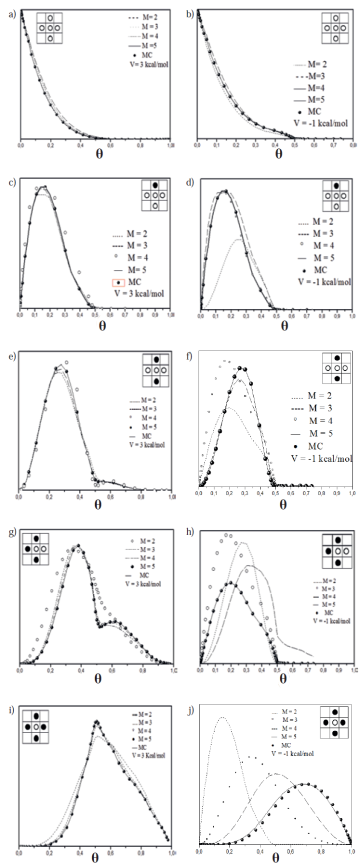
Figure 1 Correlations obtained by Monte Carlo and Transfer Matrix for repulsive and attractive values of the lateral interaction. 

The results showed the expected behavior, regardless of the lateral interaction, the matrix size is predominant in matching both methods, which is reached just for values of M = 5. This previous study of the correlations, allowed to determine the size of the matrixes to calculate observables by TMM, regarding the normalized sticking coefficient obtained by MC can be considered as a reference because it was found (27) how these experiments leads to the same result as that obtained by accurate analytical methods for dimension and its simple extension to two dimensions leads to an efficient way to get this results, which are shown in Figure 2a) and b) respectively, it can be seen that, both for a soft dynamic (Kinetics of interaction) to a hard dynamic (kinetic Ising) differences between the two methods chosen is practically null when M = 5. As mentioned previously, the correlation between the results by both methods was accurate for all dynamic schemes.

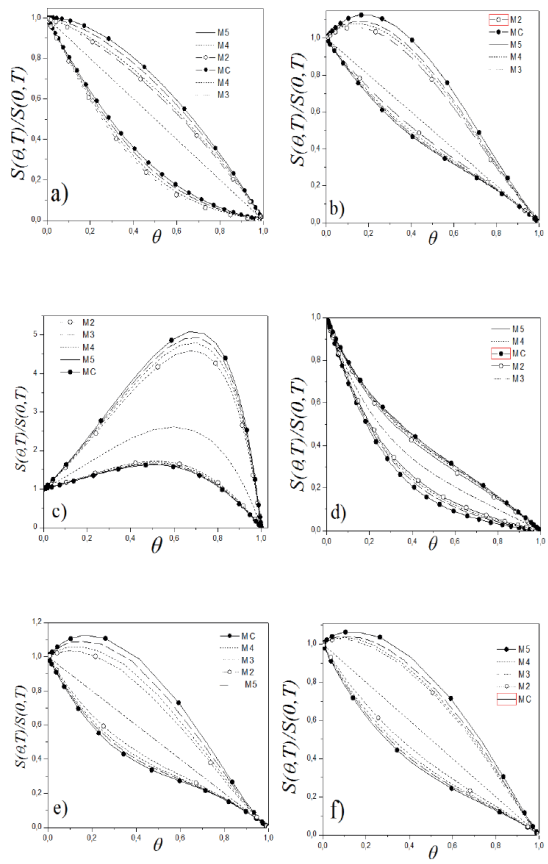
Figure 2 Sticking coefficient normalized to the dynamic scheme, a) Interaction Kinetic, b) TST, c) Inverse Relation, d) Soft Glauber, e) Ising, and f) TDA; Obtained with MC and TMM. 

TPD with MC and TMM. As mentioned, the TMM method is used for calculations in equilibrium, therefore it can only be obtained for mobile TPD (Figura 3). This is the reason why only the spectra were compared with mobile adsorbate desorption with both methods for dynamic schemes hard and soft, with zero, attractive and repulsive interactions, and θ = 0.1 to 0.9 covering. With the same criteria as for the previous observable, we chose some dynamic schemes not to extend the reading unnecessarily.

Figure 3 TPD a) and b) Ising kinetics, c), d) and e) Interaction kinetics, e) and f) Inverse relation and h) TST. In all cases for coverings from θ=0.1 to 0.9 

Conclusions

This paper presents a study in two dimensions on the influence of the different dynamic schemes proposed in the observable. Due to the inability to obtain the exact solution for covering and correlation functions, simulations for observables were presented by two different methods, Monte Carlo and transfer matrix, the fit between both methods was accurate for the sticking coefficient for all dynamic schemes studied. The spectra obtained by thermal programmed desorption Monte Carlo simulations and Transfer Matrix agree acceptably within the finite size effects.

Is a high influence of the dynamics in the process, with a different behavior depending on whether hard or soft kinetics. When the lateral interactions increase the thermodynamic limit approximation of deterioration, especially in the attractive case. However, the temperature ranges in which the desorbed system, the maxima and minima of the curves, are independent of the method used.

The matrix computation times for transfer matrix are few minutes fast information provided substantially shortened intervals typical Monte Carlo calculation, which are usually of hours. Although with the same rectangular geometry, it is noted that the simulation was carried out in square sites grids 100 side, while for TMM, the grids are endless bands up to 10 rows.

To this can be attributed some of the most differences, to corroborate TPDS were made on elongated grids (L> 400) with the same number of rows TMM, being total agreement between the curves.

This limitation (TMM) method can reduce exploiting the invariance of the Hamiltonian model (translational imposing periodic boundary conditions) reducing matrices tools Group Theory.