1. Introduction

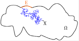
Over the last few years there has been growing interest in understanding the relationship between the geometry of a domain in Euclidean space and the properties of the solutions to canonical partial differential operators defined on it. The question of whether the boundary behavior a general harmonic function can distinguish between a ball and a snowflake or between a Lipschitz domain and the complement of the 4-corner Cantor set illustrates the type of issues one is concerned with in this area of analysis, which lies at the interface of Partial Differential Equations, Harmonic Analysis, Geometric Measure Theory and Free Boundary Problems (figure 1).

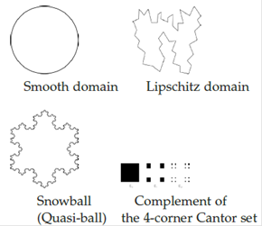
From the geometric point of view the boundaries of these four domains are very different. A smooth domain in R ⁿ is, locally, the area above the graph of a C^∞ function, tangent planes exist and are continuous at each point of the boundary, the (n − 1)-dimensional Hausdorff mea-sure, H ^{n −1}, of a surface ball (that is a ball centered on the boundary intersection the boundary) of radius r grows like ^{_rn −1} for r small. A Lipschitz domain in R ⁿ is, locally, the area above the graph of a Lipschitz function, tangent planes exist H ^{n −1} almost everywhere on the boundary, the (n − 1)-dimensional Hausdorff measure of a surface ball of radius r grows like ^{_rn −1} for r small. A snowball (resp. a typical quasi-ball, that is the image of the unit ball by a quasi-conformal map on the whole space) is not locally the area above any function, tangent lines (resp. tangent planes) do not exist and the H¹ (resp. H ^{n −1}) measure of surface balls is infinite. Furthermore for a typical quasi-ball in R ⁿ the Hausdorff dimension of the boundary is strictly greater than n − 1. The complement of the 4-corner Cantor set (produced by iterating the picture above) has a totally disconnected boundary of Haus-dorff dimension 1, the H¹ measure of a surface ball centered on the boundary and of radius r grows like r for r < 1. On the other hand since the 4-corner Cantor set is purely unrectifiable tangent lines do not exist on any subset of positive H¹ measure.

Nevertheless from the analytic point of view, under the correct magnifying glass, these domains are very similar. In fact these four type of domains are uniform or 1-sided NTA (non-tangentially accessible, see Definition 2.4) and satisfy the CDC (Capacity Density Condition)(see (^Ma), (^A1), (^A2), (^HM1), (^HMT2)). The CDC is a rather technical condition, which will not be defined here. The reader should interpret it as a uniform measure of the thickness of the complement of the domain which makes the domain Wiener regular (see (^W) and Definition 1.1) and yields additional estimates on the continuity of the classical solution to the Dirichlet problem if the boundary data f is Lipschitz.

Definition 1.1. A bounded domain Ω ⊂ R ⁿ is said to be Wiener regular for L if for any f ∈ C(∂Ω) there exists u ∈ W^1,2(Ω) ∩ C(Ω‾) satisfying

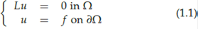
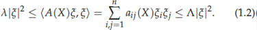
where Lu = −div (A(X) ∇u) and A(X) = ( ^_aij (X)) is an uniformly elliptic matrix with bounded measurable coefficients, i.e. there exist 0 < λ ≤ Λ < ∞ such that for X ∈ Ω and ζ ∈ Rⁿ

Remarks 1.1. (1) If A = Id, then L = ∆ is the Laplacian. In general L is a variable coefficient version of the Laplacian. A domain Ω is Wiener regular for L if and only if it is Wiener regular for the Laplacian ((^LWS)).

(2) Lu = 0 means that u and its weak derivatives are in L ²(Ω) and that for any ζ ∈ C¹ _c (Ω)

(3) The maximum principle holds for the solutions to (1.1),

(4) The interior regularity is a classical result due to DeGiorgi, Nash and Moser: u is Hölder continuous in Ω (see (^DeG), (^N), (^Mo)). Furthermore additional regularity of A implies higher interior regularity of the solution (see (^GT)).

(5) If Ω is regular then for X ∈ Ω and f ∈ C(∂Ω) if u ∈ C(Ω‾) is the solution to (1.1), by the Maximum Principle |u(X)| ≤ max_∂Ω |f|. Thus for each X ∈ Ω, the operator ^_TX : C(∂Ω) → R defined by ^_TX (f) = u(X) is a bounded linear operator, with || ^_TX || ≤ 1. Moreover ^_TX (1) = 1. Hence by the Riesz Representation Theorem there is a probability measure ω ^_XL s.t.

ω ^_XL is the L−elliptic measure of Ω with pole X.

(6) If L is the Laplacian ω _L = ω is the harmonic measure. For a domain Ω ⊂ R ⁿ , ω ^X (E) denotes the probability that a Brownian motion starting at X will first hit the boundary at a point of E ⊂ ∂Ω (see figure below). As a function of X, ω ^X (E) is a harmonic function.

(7) If Ω is (Wiener) regular and connected the Harnack principle implies that for X, Y ∈ Ω, ω ^_XL and ω ^_YL are mutually absolutely continuous. In fact given a compact set K ⊂ Ω and E ⊂ ∂Ω, ω ^X (E)/ ω ^Y (E) is bounded above and below by a constant depending only on n and K. This makes the type of properties we focus on are independent of the pole X so we denote ω ^X simply by ω.

One of the sample questions in this area is whether the harmonic measure distinguishes between: smooth domains, Lipschitz domains, quasi-balls or the complement of the 4-corner Cantor set? This is part of a central theme which addresses the problem of characterizing the operators L satisfying (1.2) in a uniform domain Ω ⊂ R ⁿ with Ahlfors regular boundary (see Definitions 2.4 and 2.5) for which the behavior of the elliptic measure determines the structure of the ∂Ω.

2. The Laplacian on non-smooth domains

In this section we consider different classes of Wiener regular non-smooth domains: Lipschitz domains, uniform domains with Ahlfors regular boundaries (these are a special type of uniform domains satisfying the CDC, see Definition 2.1 or (^A1), (^A2) and (^Z)), non-tangentiallly accessible (NTA) domains (see Definition 2.4) and chord-arc domains (see Definition 2.6).

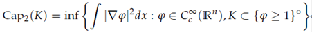
Definition 2.1. A domain Ω ⊂ R ⁿ with n ≥ 3 is said to satisfy the capacity density condition (CDC) if there exist constants c ₀, R > 0 such that for any q ∈ ∂Ω and any r ∈ (0, R), we have

For any compact set K, Cap₂(K) is defined as follows:

Definition 2.2. (^JK) A domain Ω ⊂ R ⁿ satisfies the Corkscrew condition if for some uniform constant c > 0 and for every surface ball ∆ := ∆ (q, r) = ∂Ω ∩ B(q, r), with q ∈ ∂Ω and 0 < r < diam ∂Ω, there is a ball B(X∆, cr) ⊂ B(q, r) ∩ Ω. The point X _∆ ⊂ Ω is called a corkscrew point relative to ∆.

Definition 2.3. (^JK) A domain Ω satisfies the Harnack Chain condition if there is a uniform constant C such that for every ρ > 0, Λ ≥ 1, and every pair of points X, X’ ∈ Ω with δ(X), δ(X’) ≥ ρ and |X - X’| < Λρ, there is a chain of open balls B ₁, . . . , ^_BN ⊂ Ω, N ≤ C(Λ), with X ∈ B ₁, X’ ∈ ^_BN , ^_Bk ∩ _{^Bk +1} ≠ ø and C ⁻¹ diam ^_Bk ≤ dist ( ^_Bk , ∂Ω) ≤ Cdiam ^_Bk . The chain of balls is called a Harnack Chain.

Definition 2.4. A domain Ω is a 1-sided NTA or uniform domain if it satisfies both the Corkscrew and Harnack Chain conditions. Furthermore, we say that Ω is an NTA domain if it is 1-sided NTA and if, in addition, Ω _ext: = R ⁿ \ Ω‾ also satisfies the Corkscrew condition.

Definition 2.5. Given a domain Ω ⊂ R ⁿ , we say that ∂Ω is Ahlfors regular if there is some uniform constant C such that

for all q ∈ ∂Ω and 0 < r < diam ∂Ω.

Definition 2.6 (1-sided CAD and CAD). A 1-sided chord-arc domain (1-sided CAD) is a 1-sided NTA domain with Ahlfors regular boundary. A chord-arc domain (CAD) is an NTA domain with Ahlfors regular boundary.

Remarks 2.1. (1) Smooth domains, Lipschitz domains and quasi-balls are NTA domains.

(2) CAD have uniformly rectifiable boundaries (see (^DS1), (^DS2) for definitions and relevant results).

(3) Bounded Lipschitz domains are CAD.

We discuss the extent to which the harmonic measure distinguishes between these types of domains. Here is a sample of the questions we ask.

(1) What properties of ω depend on the geometry of Ω and more precisely on the fact that Ω is a uniform domain with Ahlfors regular boundary?

(2) In this case what is the relationship between σ and ω?

(3) Does the behavior of ω with respect to σ determine the geometry of the boundary?

To illustrate the type of results we have in mind we cite below a couple of authors who laid the foundation of what has become a booming field.

In 1970 Hunt and Wheeden (^HW) proved that on a bounded connected Lipschitz domain the harmonic measure ω is doubling, i.e. there exists a constant C > 0 such that for all q ∈ ∂Ω and 0 < r < diam Ω

In 1977 Dahlberg (^D1) showed that on a bounded Lipschitz domain ω « σ and ω ∈ B ₂(σ), i.e. the Radon-Nikodym derivative of ω with respect to σ, k = dω/dω satisfies a reverse Hölder inequality with exponent 2. More precisely for q ∈ ∂Ω and r ∈ (0, diamΩ)

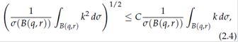
where k = dω/dω is the Poisson kernel. In particular ω ∈ A _∞(σ) = ^_Up >1 ^_Bp (σ), which means that ω and σ are quantitatively mutually absolutely continuous.

Motivated by the work in (^HW) in 1982 Jerison and Kenig (^JK) introduced the notion of NTA domains and proved that on an bounded NTA domain: 1) the elliptic measure ^_ωL of L as in (1.2) is doubling; 2) the non-tangential limit of the solution of (1.1) at the boundary exists and coincides with ^{_{f ωL}} -a.e (i.e u = f on ∂Ω), if f is Lipschitz, u is Hölder continuous in Ω‾; 3) the uniform boundary Harnack principle holds, i.e. the ratio of 2 non-negative solutions which vanish on an open piece of the boundary is bounded and 4) CFMS (CFMS) holds: i.e. the density ratio of elliptic measure is comparable to the “normal derivative" of the Green function toward the boundary. These four properties were known to hold on Lipschitz domains but the fact that they held independently of the differential structure of the boundary raised many questions (^KT1). In 2004 Aikawa (^A1) provided a characterization of uniform domains with CDC in terms of the boundary behavior of harmonic functions and harmonic measure. Aikawa’s results fit in the free boundary regularity theory as they describe the geometry of the domain in terms of the canonical harmonic functions associated to it. To some extent this is the converse problem than the one studied in (^JK). In (^HMT1) the authors show that the results (^JK) can be extended to uniform domains satisfying the CDC. Thus in particular to uniform domains with Ahlfors regular boundaries (see (^Z)).

Dahlberg’s work raised a fundamental question: on a Lipschitz domain, for what type of operators L = −div(A∇) where A satisfies (1.2) is ^_ωL ∈ A _∞(σ)? Examples appeared in (^MMS) and (^MM) exhibit Lipschitz domains and operators L for which ^_ωL and σ are mutually singular. In (^CFK) the authors provide a characterization of operators with continuous coefficients on the unit ball for which ^_ωL and σ are mutually absolutely continuous. Dahlberg’s work and these examples generated a wealth of activity which would be described briefly in Section 3.

The first results generalizing Dahlberg’s result concerning harmonic measure to non Lipschitz domains appeared in (^DJ) and (^S) where the authors proved that if Ω is a CAD then the harmonic measure ω ∈ A _∞(σ). As the field has evolved, the focus has turned to the question of what does the fact that ω ∈ A _∞(σ) imply about the geometry of Ω? Very recently several authors have started also looking at the question of what geometric information about Ω is encoded in the fact that ^_ωL ∈ A _∞(σ) and whether this depends on the operator L. See Section 3.

We finish this section by highlighting a couple of recent results in this area concerning the relationship between the properties of the harmonic measure and the geometry of the boundary. The first one provides a necessary and sufficient condition for quantitative absolute continuity (in the form of the ^_A∞ property) of harmonic measure with respect to surface measure. The second provides a sufficient condition (in terms of the behavior of harmonic measure with respect to surface measure) to guarantee rectifiability, which should be understood as a statement about the regularity of the boundary. In fact, E ⊂ R ⁿ , is rectifiable (more precisely (n − 1)-rectifiable) if it can be included in a countable union of Lipschitz images of R ^{n −1} union a set of H ^{n −1} measure 0 (see (^EG)). Uniform rectifiability is a quantitative version of rectifiability (see (^DS1), (^DS2)).

Theorem 2.1. Suppose that Ω ⊂ R _{^{n is a uniform domain, with Ahlfors regular boundary. Then the following are equivalent:}}

(1) ∂Ω is uniformly rectifiable.

(2) Ω is an NTA domain, and hence, a chord-arc domain (CAD).

(3) ω ∈ A _∞(σ).

As mentioned above, the implication (2) ⇒ (3) was proved independently in (^DJ) and in (^S), while (3) ⇒ (1) appears in (HMU), and (1) ⇒ (2) was proved in (^AHMNT).

Theorem 2.2. (^AHMMMTV2) Given an open connected set Ω ⊂ R ^{_{n, and E}} ⊂ ∂Ω with H ^{n −1} (E) < ∞ absolute continuity of the harmonic measure ω with respect to the Hausdorff measure restricted to E (i.e. ω « H ^{n −1} └ E) implies that ω └ E is rectifiable.

For further information of the type of research carried forward in this area see also (^AHMMMTV1), (^ABHM), (^HL), (^HLMN), (^HM1), (^HM2), (^HMM), (^HMMTV), (^KT1), (^KT2), (^KT3).

3. Second order divergence form elliptic operators on non-smooth domains

In this section we describe some of the contributions to the problem of characterizing the operators L for which ^_ωL ∈ A _∞(σ). There are several distinct approaches to this question.

The first approach begins with the work of Dahlberg, (^D2), and involves the perturbation theory for elliptic operators on Lipschitz domains. The initial observation is that if two uniformly elliptic second order divergence form operators L ₀ = −div(A ₀ ∇) and L ₁ = −div(A ₁ ∇) coincide in a neighborhood of the boundary of a Lipschitz domain Ω (i.e. A ₀ = A ₁ near ∂Ω) then ω ₀ ∈ A _∞(σ) if and only if ω ₁ ∈ A _∞(σ). Here ^_ωi is the elliptic measure of ^_Li in Ω. In (^D2) the author showed that on a Lipschitz domain Ω if the deviation function, defined by,

where δ(X) is the distance of X to ∂Ω, satisfies

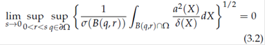
then ω ₀ ∈ A _∞(σ) if and only if ω ₁ ∈ A _∞(σ). Dahlberg’s proof is very ingenious and has been used successfully to refine his results (see (^E) and (^MPT2)). Nevertheless the fact the hypothesis included a smallness assumption (that is that the limit as s → 0 of the above quantity be 0) puzzled the experts for some time. In 1991 R. Fefferman, Kenig and Pipher showed, using techniques from harmonic analysis, that the smallness condition is not necessary. The following definition allows us to state this important result.

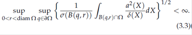
Definition 3.1. Let Ω be a uniform domain with Ahlfors regular boundary. Let L ₀ = −div(A ₀ ∇) and L ₁ = −div(A ₁ ∇) be such that A ₀ and A ₁ satisfy (1.2), L ₁ is a perturbation of L ₀ if

Theorem 3.1. (^FKP) Let Ω be a Lipschitz domain. Let L ₁ be a perturbation of L ₀ then ω ₁ ∈ A _∞(dσ) if and only if ω ₀ ∈ A _∞(dσ).

Currently similar results are available for CAD (^MPT1). On going work indicates that they also hold on uniform domains with Ahlfors regular boundaries. See (^CHM) and (^AHMT).

Other approaches to the question of whether the elliptic measure ^_ωL on a Lipschitz domain or a CAD is an ^_A∞ -weight with respect to σ, focus on either the behavior of solutions with specific boundary data ((^DKP), (^Z), (^KKiPT)), the structure of A (see for example (^KKoPT), (^HKMP), (^KKiPT)) or the oscillation A. In terms of the oscillation the key point is to control the behavior of A near the boundary. We present below a result that illustrates this well.

Theorem 3.2. (^KP) Let Ω ⊂ R ^{_{n be a connected Lipschitz domain. Let A}} (X) = (ai,j(X))_{1≤ i , j ≤ ^{n be a real matrix such that ai}} ,j ∈ ^_L∞ (Ω) for 1 ≤ i, j ≤ n, and A is uniformly elliptic (see (1.2)) Suppose further that A satisfies the following conditions:

(a) || |∇A| δ|| _{L∞ (Ω)} < ∞, where δ (X) = dist (X, ∂Ω).

(b) ∇ A satisfies the Carleson measure estimate:

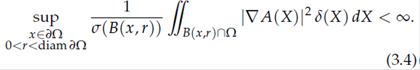
^{_{Then ωL}} ∈ A _∞(σ).

Using the work in (^DJ) a simple argument shows that Theorem 3.2 also holds on CADs. A central question in the field, which is under active investigation, is whether for operators satisfying the hypothesis of Theorem 3.2, a characterization like the one provided in Theorem 2.1 holds. The proof of Theorem 2.2 depends very deeply on the fact that the operator is the Laplacian, efforts are underway to prove similar results for more general operators using tools from Geometric Measure Theory rather than Harmonic Analysis. See (^HMT2), (^AGMT), (^TZ).