1. Introduction

A correct determination of magnetic nanoparticle (MNP) properties is important for determining their best field of application [¹]. These properties must be studied directly in the supporting matrix containing the MNP, because inter-particle interactions (such as dipolar magnetic, electrostatic or steric), can produce MNP structuring. In this way MNP properties, influenced by the environment, are modified, and must be taken into account especially if the MNP will be used for biomedical applications [²-⁴].

The imaging techniques usually used to characterize the morphology of MNP, such as Transmission Electronic Microscopy (TEM), Scanning Electronic Microscopy (SEM) or Atomic Force Microscopy (AFM), don’t provide direct evidence of the particle structuring, especially when the MNP are supported in a liquid matrix as used for biomedical applications. In microscopy techniques, the sample is diluted and dropped in a sample-holder and dried to evaporate the liquid matrix, inducing particle aggregation in a different way than that expected in concentrated suspensions. A better alternative could be Cryo-TEM, in which the sample is quickly frozen using liquid nitrogen, keeping the MNP structuring [⁵], nevertheless, as with TEM, the sample must be diluted, diminishing the influence of the distance-dependent interactions among particles [⁶-⁸].

The presence of MNP structures in liquid suspensions can be estimated using scattering techniques, where the scattering pattern can be modelled using a form factor that gives information about particle size and morphology, and a structure factor, that gives information about how particles are spatially assembled [⁹].

In this context, the Small Angle X-ray Scattering (SAXS) technique is a powerful tool to investigate the MNP structuring in a viscous liquid matrix. In this technique, the sample is illuminated with a monochromatic x-ray beam of wave-length λ. The x-rays interact with the particle’s electrons producing scattered radiation. The intensity of the scattered radiation (I) depends on the scattering angle θ, usually between 0.01 and 0.07 rad, as expressed in eq. (1).

where the scattering vector , and the electronic scattered intensity where is the electronic density difference and V _p is the particle volume, and V _p is the form factor.

Assuming spherical particles with a size distribution g(R) the scattered intensity, including a structure factor S(q) can be written as expressed in eq. (2):

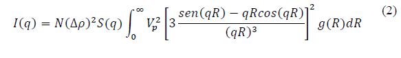
This way to take into account the structure factor is called a monodisperse approach and is the simplest way to include a structure factor in the analysis. This approach simply multiplies the size-averaged form factor with the structure factor. Here it is assumed that the interaction potential between particles are spherical symmetric and independent of the particle size [¹⁰].

The use of eq. (2) has been successfully used to fit the SAXS data retrieved from scattering patterns produced by nanoparticles in suspension. In addition to the particle shape and particle size distribution, the MNP structuring also can be inferred from the correct choice of S(q) and analysis. [⁹,¹¹-¹³].

The correct determination of aggregation using SAXS depends on choosing the correct mathematical model, this means that all the -parameters used must have physical significance and their value must be consistent with the measurement range in use.

The aim of this work is to understand the structuring of magnetic nanoparticles in colloidal suspensions using SAXS. Additionally, a methodology to analyze SAXS patterns is also proposed.

SAXS patterns obtained from two different Fe₃O₄ nanoparticles colloidal suspensions are used to determine the particle shape and size distribution. The structure is determined using two different mathematical models for S(q): mass fractal and hard sphere. While the mass fractal mode gives information about how particles are structured (chain, planar or spherical), the hard sphere model gives information about how compacted the aggregates are.

Results are compared and used to determine how interactions among particles structure the colloidal suspension and could be applied for understanding the structure of nanoparticles in different viscous matrices, providing a useful method for studying SAXS patterns in which the use of structure factors is necessary.

2. Methodology

Fe₃O₄ nanoparticles were synthesized using the co-precipitation method [¹] at 60ºC. To stabilze them in an aqueous medium, a citric acid solution (0.2 g/ml) was added to the as-synthesized particles until pH = 4.6 was reached. The mixture was stirred for 90 minutes at 60ºC. The pH of the final solution was around 7 and the volume was fixed at 50 ml.

The colloid was gravitationally decanted, resulting in two different samples, the first, labeled as S1, corresponds to the supernatant, composed of the smaller and better-stabilized particles in suspension, and the second, labeled as S2 corresponds to the pellet, composed of the bigger and less-stabilized particles precipitated at the bottom of the vessel. The shape and size of the particles was first determined using transmission electronic microscopy (TEM).

SAXS patterns were taken in the National Laboratory of Synchrotron Light (LNLS) at Campinas-Brazil, using monochromatic x-ray radiation with λ = 1.822 Å. The 2-D scattering patterns were recorded using a MAR165-CCD camera. In order to achieve a q-range of 0.06-4 nm^-1 two sample-detector lengths were used (975 and 1977 mm). SAXS pattern of water was used to join the data coming from the two lengths and to express data in absolute units (cm^-1) of the differential scattering cross section (dΣ(q)/dΩ).

SAXS patterns were fitted using Eq. (2) and the size distributions g(r) were retrieved. In order to analyze the particle structure of the samples, two procedures were employed. In the first one, global scattering functions were used for data modeling. This model, named the Beaucage model, considers approximations of Eq. (2) when q → 0 and q → ∞, resulting in a sum of Guinier and Porod functions. The second method consists in fitting Eq. (2) using two different S(q) models: a mass fractal structure factor (S _f (q)) and a hard sphere structure factor (S _HS (q)).

3. Results

In Fig. 1, TEM images of both samples are shown. Images reveal that particles are mostly spherical. After counting around 100 particles the radius (R±s.d, s.d. being the standard deviation) of sample S1 is 4.5±1.0 nm and for sample S2 is 5.5±1.1 nm. As expected, the decantation process results in two different mean size samples.

Source: The Authors.

Figure 1 TEM images for samples (a) S1 (well-stabilized sample) and (b) S2 (poorly-stabilized sample). 

SAXS patterns were taken for both samples following the procedure described in the previous section. Typical two dimensional scattering patterns are shown in Fig. 2.

Source: The Authors.

Figure 2 

The intensity is azimuthally integrated in order to obtain a one-dimensional SAXS pattern as shown in Figure 3. Water scattering patterns were used to express SAXS intensity data (originally expressed in arbitrary units) in the units of differential scattering cross section (dΣ(q)/dΩ).

Source: The Authors.

Figure 3 One-dimensional SAXS patterns obtained for samples (a) S1 and (b) S2. Continuous lines represents the best fit obtained using the Beaucage model. In (a) the contributions of each term of the model are shown. 

3.1. Global scattering function: beaucage model

In order to obtain structural information from the SAXS patterns, data were fitted using the Beaucage model as expressed in Eq. (3).

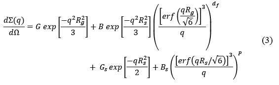
Where, R _s is the particle Guinier radius, R _g is the cluster Guinier radius, G and G _s are the pre-exponential Guinier coefficients for the clusters and the particle respectively, B and B _s stand for the pre-exponential Porod coefficient for the cluster and the particle respectively, d _f is the aggregate fractal dimension and takes values between 1 and 3, being 1 a lineal aggregate and 3 a spherical aggregate, and P = 4 is the Porod exponent.

The fitting parameters obtained using this models are shown in Table 1.

Table 1 Fitting parameters for samples S1 and S2 using the Beaucage model. R _s is the particle Guinier radius, R _g is the cluster Guinier radius, G and G _s are the pre-exponential Guinier coefficients for the cluster and the particle respectively, B and B _s stand for the pre-exponential Porod coefficient for the cluster and the particle respectively, d _f is the aggregate fractal dimension. 

Source: The Authors.

Results show that particles are aggregated in both samples, and bigger aggregates are observed for sample S2, it is consistent with the fact that the S2 sample is composed of poorly-stabilized particles, and the particles’ aggregation is due the magnetic dipolar interaction. As it is know, magnetic dipolar interaction is an anisotropic interaction, resulting in chain conformation. It is possible to deduce from SAXS using the fractal exponent (d _f ), the value of 2.43 for sample S2, which indicates a broad ramified structure and the value 2,97 indicates a more spherical compacted structure.

The particle radius can be calculated from R _s using the expression resulting in 4.1 nm and 5.0 nm for samples S1 and S2 respectively, in accordance with measured by TEM.

Once the model was fitted, the contribution from each term in Eq. (3) was also plotted for sample S1, as shown in Fig. 3, indicating that the first and second term in Eq. (3) contribute to the scattering at lower q-values and the third and fourth term contribute to the higher q-values. In this way, is possible to confirm the evidence for particle aggregation in the lower range of q-values.

3.2. Form factor and structure factor determination

Once the size and aggregation parameters have been defined using the Beaucage model, now is important to determine the particle shape (form factor) and the structure factor. For this, Eq. (2) was fitted to SAXS data for samples S1 and S2. Results using are shown in Fig. 4(a) . Here we see that considering only the form factor is not sufficient to fit the experimental SAXS data.

First at all, a mass-fractal structure factor was used in order to fit the complete experimental SAXS data. The mass-fractal structure factor assumes that the lower q-values scattering pattern can be modelled using a power law, so that, the exponent represents the fractal dimension, this range of values is limited by finite cluster size (ξ) and by the primary particle size (R), by means of an exponential cut-off pair correlation function [¹⁰].

The mass-fractal structure factor can be expresed as:

Where Γ is the gamma function.

In this way, experimental SAXS data were fitted using Eq. 2 and Eq. 4 with a LogNormal radius distribution (g(R)). Fitted parameters were the median radius (R _o ), the standard deviation (σ) of the of the variable ln(R/R _o ), the aggregate size (ξ) and the fractal dimension (d _f ). The mean particle radius is calculated as .

Fitted curves are shown in Fig. 4 and fitted parameters are presented in Table 2.

Source: The Authors.

Figure 4 SAXS patterns for samples S1 and S2. (a) Fitted with only the spherical form factor and (b) Fitted with the spherical form factor and the mass-fractal structure factor. Inset in (b) shows the structure factor determined experimentally. 

Table 2 Fitting parameters for samples S1 and S2 using the sphere form factor and mass Fractal structure factor. R _o is the median radius, σ is the standard deviation of the variable , ξ is the aggregate size and d _f is the fractal dimension . Is the mean particle radius. 

Source: The Authors.

Results show that considering a mass-fractal structure factor is enough to fit all the experimental data.

The obtained fitted parameters are in the same order of magnitude that values measured with TEM and using the Beaucage model. The differences could be attributed to the used model.

Once the curves are fitted, it is possible to experimentally determine the structure factor as , where I _exp represents the experimental SAXS data and I _sph is the spherical form factor calculated using the fitted parameters listed in Table 2. The S(q) thus calculated is shown in the Fig. 3 inset, where typical structure factor behaviors are observed. For higher q-values S(q) =1, here no influence of particle structuring is observed, so this part of the scattering pattern is governed by single particle scattering. For lower q-values, the particle structuring governs the scattering pattern.

Due to particle aggregation, it is possible that particles feel an interactive energy potential. It is possible to use the sticky hard sphere structure factor to determine if this potential is attractive or repulsive.

This model considers a potential U(r) expressed as:

Where R _o is the particle radius, Δ is the interparticle distance and τ is the stickiness parameter. If , the potential is attractive, and if the potential is repulsive.

For this case, the structure factor is:

Where:

Here and:

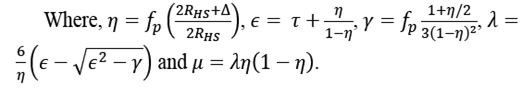
Table 3  Fitting parameters for samples S1 and S2 using the using the sphere form factor and mass hard sphere structure factor. R _HS is the hard sphere radius, τ is the stickiness parameter, and f _p is the particle volume fraction.  

Source: The Authors.

SAXS experimental data were fitted using Eq. 2 and Eq. 5 as the structure factor, adding the hard sphere radius (R_HS) and the particle volume fraction (f _p ) as fitting parameters. Best fit parameters are shown in Table 3.

As observed in Table 3, the obtained size distribution is similar to that obtained with TEM and the mass-fractal model. The fitted values for τ indicate that the particles are subject to attractive forces, as expected for magnetic nanoparticles. The fact that indicates that the particles are in contact. For sample S2 , it could be explained considering that one particle can obscure other particles, consistent with a higher packing structure as determined by the mass-fractal analysis, where d _f =2.92 for sample 2, indicating an almost spherical aggregation, in contrast to sample S1 for which d _f =2.00, indicating a ramified chain-like aggregation.

Eqs. (4)-(5) were used to simulate the structure factor using the parameters listed in Tables 2 and 3. Results (shown in Fig. 5) are similar to the S(q) determined graphically, shown in inset of Fig. 4(b), indicating that the use of the mass fractal and hard sphere structure factors are applicable to study the aggregation of particles in liquid suspensions.

Source: The Authors.

Figure 5 Simulated structure factor (S(q)) for samples S1 and S2. MF stands for mass-fractal simulations S(q) and HS stands for hard sphere simulations S(q). 

4. Conclusions

Knowledge of the nanoparticle structuring in aqueous suspensions is necessary in order to determine the applicability of such suspensions. Small Angle X-ray Scattering patterns are a good tools, widely used to determine nanoparticle structuring. Its success relies on the correct selection of the mathematical model used to fit scattering data. SAXS patterns analysis of both colloidal suspensions reveals that the better stabilized colloid is composed of smaller nanoparticles in comparison with the less stabilized colloid. The results show that the aggregation is higher in the less-stabilized colloid having bigger particles, this because the bigger the particle the stronger the magnetic dipolar interaction. For the better-stabilized colloid, particles are aggregated in 2-dimensional structures, for the less-stabilized colloid an almost spherical aggregation was determined. The fitted hard sphere radius values, determined with hard sphere model, confirm that the particles in colloid S1 are more separated and that particles in colloid S2 are more compacted. The structural data obtained with SAXS modelling are in agreement with the parameters measured using TEM, validating their use.