


 English (pdf)
 Article in xml format
 Article references
 Send this article by e-mail
 Cited by SciELO
  Cited by Google
  Similars in
SciELO
Similars in
SciELO  Similars in Google
 Permalink
1. Introduction
Remote sensing image classification is a digital process that is frequently used to create thematic cartography depicting the terrestrial land surface, as it produces reliable maps of a range of features, at different spatial and temporal scales [1]. Biodiversity, urbanization, agriculture and risk assessment studies, among others, have benefited from remote sensing-based thematic cartography [2,3,4].
Globally, thematic cartography became more important at the end of the 1980s and the years that followed with the inauguration of the European CORINE (Coordination of Information on the Environment) program. This resulted in the definition of the Corine Land Cover (CLC) methodology, a consistent and standardized set of principles, rules and procedures for obtaining thematic information for the European territories. The CLC methodology relies on the interpretation of satellite images, supported by auxiliary information, to classify remotely-sensed data into different categories at different levels of spatial detail. Auxiliary information from field surveys and secondary sources is essential to help identify and confirm the content of certain land cover characteristics that have been detected in the images [5,6,7].
In Colombia, the CLC methodology has been adopted - with minor modifications - as the standard methodology for land cover mapping by Instituto Geográfico Agustín Codazzi (IGAC) and Instituto Colombiano de Estudios Ambientales (IDEAM) [8]. The CLC methodology has been applied in a series of mapping projects at different scales and levels of detail [9].
Remote sensors are usually classified as either active (optical), which depend on sunlight; or passive (radar), which emit their own energy. Of the available information from optical sensors, the Landsat satellite mission data has been the most used by medium-spatial scale projects for land cover mapping, as well as by high spatial scale projects that have used their aerial photographs. Optical sensors have some important limitations, in particular, data collection can be hindered by atmospheric conditions, especially in areas that have cloud cover most of the year [10].
As a way round this, active sensors such as synthetic aperture radar (SAR) instruments can take images of the Earth’s surface no matter the atmospheric conditions, and can operate in cloudy conditions and in darkness. Furthermore, SAR images contain data related to surface texture and backscatter properties of land cover and, in the case of sparse vegetation, the upper substrate of the soil [10]. In sum, radar images provide more information than optical images such as the Landsat TM images [11], and their usefulness has been demonstrated by several land cover mapping studies that have used SAR images [12,13,14].
Traditional techniques for the visual interpretation of remotely sensed data, be it radar or optical data, are similar to a certain degree. However, while several studies reveal that for both data types, large amounts of information can be extracted by image interpreters, production of thematic cartography is time intensive, and requires hard work and high-level expertise [15].
The visual interpretation of images for land cover classification is based on the manual delineation of objects and shapes, and the careful observation of spatial features and geometric patterns [7]. Recent advances in software and hardware technologies, especially the design of advanced digital classification techniques, have improved the operational performance of the classification task [16]. However, several authors argue that human interpreters are still key to the land cover mapping process as they possess superior classification capabilities. This explains why digital classification procedures are heavily guided by human interpretation [16,17].
The traditional pixel-based classification techniques, used from 1980 onwards, aim to establish a quantitative and statistical relationship between pixel data and categories of interest (14). Such techniques have limitations when applied to high-spatial resolution images, available since 2000, because they focus on individual pixels which are smaller in size compared to the typical size of the elements being studied, and do not take into account spatial features such as texture, shape and context patterns [14]. Therefore, the pixel-based image analysis approach is very limited when it comes to land cover mapping using high-spatial resolution images, although these limitations can be overcome to some degree if object-based techniques are used [14].
The object-based approach for land cover classification starts by grouping pixels into image-regions, by means of a segmentation task [18] that generates discrete objects or pseudo-polygons, whose size may vary in compliance with several parameters. These include aggregation schemas which may differ depending either on image spatial resolution or the spatial scale of the final map [19].
Gao and Mas [20] compared land cover classification results from the traditional pixel-based technique and the object-oriented method, using different resolutions of SPOT-5 multispectral images. Their results showed that the object-oriented method’s thematic accuracy was 25% more accurate than the pixel-based method. Perea et al. [21] used the object-oriented method to carry out the digital classification of an urban-forest area using digital aerial photographs. They obtained a thematic accuracy of 90% and showed that image objects output from the segmentation task may also be used for a further “refined” classification [22].
Random forest is among the most efficient of the different machine learning algorithms for digital classification [23]. A random forest is a collection of hundreds of decision trees that collaborate to produce a reliable classification [23]. The outstanding feature of the random forest technique is that it provides more accurate results than other classification techniques, even when there are more variables than observations [24]. Random forest generalizes the training features well and evaluates the importance of the variables for the classification task [25]. It is also very efficient with large volumes of data [26,27].
This can be seen in the study by Balzter et al. [13], where Sentinel-1 radar images and geomorphometric variables were input into the random forest algorithm for land cover classification. It showed that it is possible to discriminate coverages with a thematic accuracy of up to 68.4%, which is useful for mapping tropical regions with frequent cloud cover. Likewise, Lawrence et al. [28] implemented random forest to discriminate two different invasive plant species, obtaining thematic accuracies of between 66% and 93%, highlighting the potential of random forest for land cover mapping.
The objective of the present study was to compare the accuracy of thematic cartography obtained using two different classification approaches, pixel-based and object-oriented, using the random forest algorithm. In the case study, both Sentinel-1 radar and Sentinel-2 optical images acquired by the European Space Agency (ESA) were used as the main input data. The land cover classifications were obtained in compliance with the CLC methodology adapted for Colombia at three levels of detail: exploratory (Level 1), reconnaissance (Level 2) and semi-detailed (Level 3). The overall aim is to evaluate the potential of Sentinel 1 and Sentinel 2 images for thematic mapping, and hence, to provide empirical evidence to support the work of national mapping agencies which are moving towards digital techniques to replace traditional mapping methods.
2. Materials and methods
2.1. Study Area
The study area is located in the department of Cundinamarca, comprising the municipalities of Facatativá, El Rosal, Madrid, Bojacá, Mosquera and Funza (see Fig. 1). Elevation ranges between 2300 and 2900 masl, with an average height of 2500 meters. Slope varies between 0% and 25% with an average of 18%. The study area covers approx. 30,000 hectares. This area was selected due to the availability of high-quality land cover information, obtained by the Colombian national geographic institute at three different spatial levels, using well-established visual techniques of image analysis.

2.2. Data
2.2.1. Images
The European Space Agency (ESA) Copernicus program is comprised of satellite missions Sentinel 1 and Sentinel 2 [29], offering operational satellite data that is useful for land cover mapping, land change detection and estimation of physical-geochemical variables [30].
Sentinel 1A operates a C-band synthetic aperture radar (SAR) instrument (5.404 GHz) which is not affected by cloud cover or lack of light. The IW (Interferometric Wide) swath mode combines a large scan width (250 km) with a moderate geometric resolution (5 m x 20 m). The IW mode is the most commonly used mode for land cover studies [31].
The Sentinel-1A (Ground Range Detecting) single-level image used was acquired on September 16, 2015. The specifications of the image (Fig. 2) are summarized in Table 1.
Table 1 Specifications of the Sentinel 1A Radar Image. V denotes vertical polarization, H denotes horizontal polarization.

Source: The Authors.
Sentinel-2A consists of two polar-orbiting satellites each with a multispectral MSI sensor (Multi Spectral Imager) of high-medium spatial resolution, characterized by a 290-kilometer wide strip and a high revisit capacity (5 days with two satellites) [32].
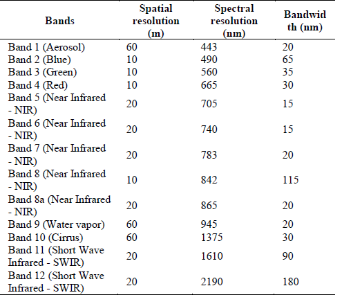
The Sentinel-2A MSI images used in this study (Fig. 2) are summarized in Table 2 [31].

Source: The Authors.
Figure 2 Study Area. Left: Sentinel 1A radar image - polarization combination VV-VH- (VV-VH). Right: Sentinel 2A optical image - color composition RGB 432.
2.2.2. Reference data
The thematic information used as reference for training and validation is a vector data produced by Instituto Geografico Agustin Codazzi (IGAC) and Corporacion Autonoma Regional de Cundinamarca (CAR). The reference dataset comprises thematic cartography in accordance with CLC methodology at scale 1:25,000, semi-detailed level, for the inter-administrative contract CAR-IGAC (1426 / 4705-2016). The reference dataset was obtained using Sentinel-2A images from 2015 and includes land cover classifications from level 1 to level 6, obtained from visual image interpretation conducted by expert cartographers at IGAC.
The CAR reference data for the study area has 41 land cover classes in level 3, 13 land cover classes in level 2, and 5 land cover classes in level 1. For the training step, approximately 10% of the total area for every class was used in order to avoid both over-training and under-training. Then, for the validation step, the remaining 90% of the area was used.
2.3. Methods
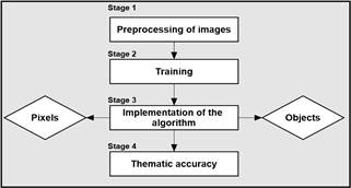
The workflow diagram shown in Fig. 3 consists of four stages: in Stage 1, radiometric and geometric corrections were conducted on radar and optical images, and the spectral variables to be analyzed were prepared; in Stage 2, training areas were established in levels 1, 2, 3; in Stage 3, the random forest algorithm was used to classify land cover in the study area, using the pixel and object-oriented techniques and identifying relevant variables to perform the integration of optical and radar data in the classifications for levels 1, 2, 3; in Stage 4, thematic accuracy was assessed for each image analysis technique implemented and for each level of classification.
2.3.1. Stage 1. Preprocessing of images
The Sentinel-1A image was calibrated in the Sigma angle of incidence, the multilooking process was applied to two ranges in order to obtain square pixels, the "speckle" or noise was corrected with the Lee Sigma filter in a 5x5 window and topographic distortion was removed using the SRTM 1 arc sec digital elevation model [14]. The digital level (DN) values of the SAR image were converted to backscattering values on the decibel scale (db). All processes were carried out in the SNAP software [14].
The polarimetric data of the Sentinel-1A image (VV - VH) were combined using the method outlined in Abdikan et al. [14], where the most accurate scenario is given using the VV, VH, (VV-VH) polarizations, and (VV / VH) and [(VV + VH) / 2] as training variables for the classification, and four additional combinations were calculated for a total of nine variables.
The variables, obtained from the pre-processing of the polarizations (VV - VH) of the Sentinel-1A radar data and used to carry out the classification of coverages, are shown in Table 3. Here we present the operations and combinations of each variable.

A Sentinel-2A image, obtained on 2015-12-21, was obtained using the Google Earth Engine platform [33]. The data from Sentinel-2A have 13 spectral bands that represent the top-of-atmosphere (TOA) reflectance values, these values were scaled by 10000.
The bands used have resolutions of 10 m and 20 m (B2 - B3 - B4 - B5 - B6 - B7 - B8 - B8a) and were implemented to calculate the Normalized Difference Vegetation Index (NDVI) [34]. The NDVI index can be used to produce a spectral index that separates the green vegetation from the ground [16]. It is expressed as the difference between the infrared and red bands, normalized by the sum of these bands: as show it in eq. (1).
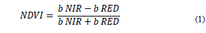
where b NIR is the infrared band TOA reflectance and b RED is the red band TOA reflectance.
The NDVI values range from -1 to 1, 1 being mature or high-density vegetation and -1 surfaces without vegetation [16].
The Enhanced Vegetation Index (EVI) optimizes the vegetation signal, improving sensitivity in regions of high biomass and reducing atmospheric influences [35]. This index is expressed as shown in eq. (2).

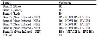
Where b is band on TOA reflectance, L is the background setting of the canopy that addresses the non-linear differential NIR and the red radiant transfer through a canopy, and C1, C2 are the coefficients of aerosol resistance, which use the blue band to correct the influence of aerosols in the red band. The coefficients adopted in the EVI algorithm are, L = 1, C1 = 6, C2 = 7.5 and G (gain factor) = 2.5 [36,37,35]. Table 4 summarizes all bands and variables implemented from the optical data.
2.3.2. Stage 2. Training
The training areas for the algorithm were extracted from the CAR 1:25000 vector information, at classification levels 1, 2, and 3. We assigned 10% of the area per class for training and the remaining 90% area for validation, as was mentioned in Section 2.2.2.
The supervised classification was implemented using the random forest learning algorithm, which uses an ensemble of decision trees as base classifiers [23]. The trees are constructed from successive binary partitions of the training data set which form subsets of homogeneity [25]. This algorithm requires predictive variables and the number of classification trees be used as input parameters; the value of 500 trees is established by default [27]. Cánovas [38] mentions that using a larger number of trees does not have a significant impact on classification accuracy.
This classification was carried out in the statistical package R using the libraries randomForest, rgdal, rgeos, sp and raster. As stated in Section 2.2.2, the CAR reference data used for the training and validation zones was produced by IGAC in 2016.
2.3.3. Stage 3. Implementation of the algorithm
The random forest algorithm can evaluate predictor variables with two parameters: the average decrease in accuracy (Mean Decrease Accuracy) and the average decrease in Gini (Mean Decrease Gini). The former measures the precision given by a variable in each random tree [25]. The latter measures the homogeneity of the variables in the random trees and is calculated each time an input variable is used to divide a node [27,39].
The classification process was carried out by implementing the random forest algorithm in two phases. In the first phase, the classification was conducted with the three levels of detail in both the pixel and object-oriented approaches, taking the optical and radar data individually. In the second phase, the parameters of (Mean Decrease Accuracy) and the average decrease of Gini (Mean Decrease Gini) were evaluated, in order to identify the best optical and radar variables, and thus, the classification was repeated with the joint data and their accuracy was compared with the individual data.
The pixel approach processing was undertaken in the statistical package R. The object-oriented approach was carried out in the ENVI 5.3 program, from which the segmentation vectors were obtained, and then classified in the statistical package R.
2.3.4. Stage 4. Thematic accuracy Assessment
For assessing thematic accuracy by classification level and by class, a vector layer of point type covering the whole study area was created using a spacing equal to the spatial resolution of the Sentinel-2A radar image (10 m) for a total of 2,699,648 points. This layer carries one attribute that represents visually identified land cover categories for the CAR-IGAC_2016 project as well as the random forest classifications at levels 1, 2, and 3. Confusion matrices were created in order to calculate Kappa indices. This stage was implemented using the fmsb, psych, foreign libraries in the statistical package R.
3. Results
3.1. Implementation of the algorithm
The algorithm evaluates the best variables using the aforementioned indices. A frequency graph was prepared (Fig. 4), in which the variables with the best index values for optical and radar data in pixel and object-oriented approaches are recorded. 5 variables of the optical data and 3 of the radar data were taken into account, these variables were those that presented the best indices according to the algorithm valuation and these data were integrated into the classifications of the pixel and object-oriented approaches. In this manner, the algorithm’s potential as a variable evaluator was measured and the accuracy obtained from the integrated optical and radar data was compared to the data when used individually in each of the implemented approaches.

As shown in Fig. 4, optical and radar data were merged as variables; B2 (Band 2 "Blue"), B3 (Band 3 "Green"), B5 (Band 5 "Near Infrared - NIR"), B8A (Band 8a "Near Infrared - NIR"), EVI_B5 (EVI calculated with Band 5) obtained from the optical data and the variables VH, ("VV - VH" / 2), (VV*VH) corresponding to the radar data.
Fig. 5 shows the results of training accuracy for the two classification approaches at levels 1, 2, and 3.
3.2. Best Classification Variables
The Sentinel-2A sensor channels that improved thematic accuracy were Band 2, Band 3, Band 5, Band 8A, and the variables that were calculated with this sensor. The study identified that the EVI calculated with Band 5 and EVI calculated with the Band 8A contributed more than the other variables and improved the classification.
Of the Sentinel-1A sensor radar data, it was clear that the VH polarization channel was the most suitable for classification, likewise, the variables obtained from this channel that improved accuracy in the resulting classification were the variable calculated from the difference between the VV and VH polarization (VV-VH) and the variable calculated from the mean of the difference between the polarization VV and VH [(VV-VH) / 2].
3.3. Thematic accuracy
The results obtained for thematic accuracy at level 1 are shown in Table 5 and Fig. 6, using the 90% of the CAR dataset, reveal that, firstly, the best global thematic accuracy is obtained from integrated radar and optical images, implementing the object-oriented approach resulting in a kappa index of K = 0.85. Secondly, we observed that the object-oriented approach applied to optical images presents with K = 0.84. Thirdly, it was found that the pixel-based approach from both optical images and integrated optical and radar images share the same accuracy at K = 0.83.


Source: The Authors.
Figure 6 Thematic Accuracy for level 1. (O.I + R.I = Optical Images with radar images.)
The results obtained from the classification at level 2 are shown in Table 6 and Fig. 7. These results reveal that the best global thematic accuracies are obtained from, firstly, the implementation of the integrated radar and optical images using the object-oriented approach, resulting in K = 0.62. Secondly, the pixel approach which used the integrated optical and radar images together with the object-oriented approach using optical images resulted in K = 0.60. Thirdly, the pixel approach using optical images produced K = 0.59. The remaining classifications obtained from the object-oriented approach with radar and pixel images show lower kappa indexes, K = 0.57 and K = 0.49 respectively.


Source: The Authors
Figure 7 Thematic Accuracy for level 2. (O.I + R.I = Integration optical and radar images.)
The results obtained from the classification for Level 3 are shown in Table 7 and Fig. 8. The combinations that demonstrated the best global thematic accuracies were, in first place, the integration of radar and optical images using an object-oriented approach resulting in K = 0.60. In second, the use of a pixel approach with optical images produced K = 0.58. In third place, the pixel approach applied to integrated optical and radar images gave K = 0.57. Fourth, applying the object-oriented approach to radar images and the pixel approach to optical images both resulted in K = 0.56. Finally, the pixel-wise approach with radar images produced K = 0.47.


4. Discussion
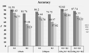
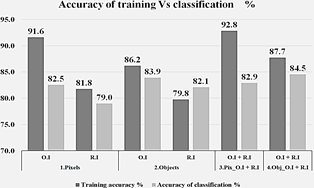
From the thematic accuracy values shown in Fig. 9, it is evident that the most informative variables are obtained from the integration of optical and radar data. Overall thematic accuracy is higher when both the pixel-based and the object-oriented approaches are applied to integrated images rather than the optical or radar datasets by themselves. The model’s accuracy when integrated data is used is approximately 10% higher than with the single datasets.
Source: The Authors.
Figure 9 Thematic accuracy vs. Training (O.I = Optical Images, R.I = Radar Images, O.I + R.I = Optical Images with Radar Images.)
The most relevant variables were: B3 (Band 3 "Green"), B5 (Band 5 "Near Infrared - NIR"), EVI_B5 (EVI calculated with Band 5) obtained from the optical data and the variables VH, ("VV - VH" / 2), (VV*VH) corresponding to the radar data. This set of variables confirm results previously obtained by Balzter [13] and Abdikan [14]. They claim that the combination of radar data with other types of variables or data can lead to greater accuracy in the classifications. The results of this study ratify the potential of RandomForest as a classification algorithm and its ability to evaluate the importance of explanatory variables [40,23].
Regarding the best approach for thematic accuracy of land cover classification, here the object-oriented technique was superior to the traditional pixel-based technique by approx. 5%, as shown in Fig. 9. This shows that the classifications obtained by applying the object-oriented technique produces higher thematic accuracy than traditional per-pixel methods [41,42,43,44].
In this study, the volume of processed data was huge, as it combined the optical data and the radar data (20 Gigabytes). Thus, it was a suitable scenario to test the high-level processing capacity of the random forest machine learning algorithm. Our results reaffirm the suitability of this algorithm for image classification, as was suggested by Balzter [13] and Abdikan [14].
The results of the classification for level 1 confirm the findings of Vargas [45,46], indicating that, for exploratory detail level where land cover is mapped on a scale of 1: 100,000, Kappa indices greater than K = 0.81 are outstanding classifications (Fig. 10).
At level 2, i.e., mapping at reconnaissance level at a scale of 1:50,000 to 1:25,000, in general, the best results were obtained by integrating radar and optical images using the object-oriented approach. Thematic accuracy corresponding to Kappa = 0.62 represents an acceptable quality (Fig. 10).

Source: The Authors.
Figure 10 Thematic accuracy for level. (O.I = Optical Images, R.I=Radar Images, O.I + R.I = Optical Images with Radar Images.)
At level 3, for mapping studies at a semi-detailed level, corresponding to scales of 1:25,000 to 1:10,000, the best results were obtained with the combination of optical and radar images using an object-oriented approach. Thematic accuracy with Kappa = 0.62 represents moderate quality (Fig. 10).
5. Conclusions
This study ascertained the performance of digital classification techniques for land cover classification. Sentinel-1 A optical data and Sentinel-2 radar data were used, both individually and in combination, for discrimination of land cover. Two different image analysis techniques, the pixel-based and object-oriented approaches, as well as the random forest algorithm, were applied to obtain land cover classes at three different spatial scales as specified by the Corine Land Cover methodology.
We obtained the best accuracy at level 1, combining optical and radar data with the object-oriented approach, and obtaining Kappa indexes greater than 0.80. This showed that the combination of optical and radar data with object-oriented classification is ideal for the identification of land cover at level 1.
Thematic accuracies decrease by an average of 19% as the level of detail and classes increases, with the “exploratory” level 1 presenting the best results for thematic mapping using the techniques, data and methods presented in this work. The thematic accuracies obtained using the object-oriented approach are superior to the pixel-based approach by 5%. In addition, it was shown that the integration of radar and optical images improves the quality of land cover mapping. To conclude, the results of this study show the potential and the limitations of using available optical and radar satellite data, as well as different digital image analysis techniques, for land cover classification at several spatial scales.

