1. Introduction
Electricity losses or operating expenses are a concern for electricity companies, since they constitute a segment of the production process that determines, among other things, quality, from the point of view of efficiency. In the case of technical losses, also called technological expenditure by some authors, their quantification attracts interest from scientists around the world due to the complexity associated with the need to process a large amount of information that is sometimes unreliable or inaccessible.
In transmission and sub-transmission networks, the economic effect of losses is extremely significant, while, in distribution networks, they hardly compensate for the expenses necessary to collect the information required for their evaluation [1,2].
In Cuba, the rate of losses fluctuates around 15%, of which 11% corresponds to technical losses, according to data provided by the Electric Union (UNE).
For the evaluation of technical losses, many researchers rely on calculation tools or computational software such as Matlab, DIgSILENT PowerFactory, among others [3-7]. These tools are mainly based on mathematical approaches such as Newton Raphson's method, Gauss Seidel or probabilistic methods for load estimates [8-11]. These methods require an accumulation of information characteristic of the system or circuit under study, which sometimes hinders or interferes with the veracity of the data, thus affecting the precision of the results. Specialists of electricity companies and some Cuban academics, dedicated to the analysis and estimation of technical losses, rely on the Radial tool, which has been implemented by a group of academics at the University of Las Villas for the studies of circuits with radial configuration. Although it is intended to change to more up-to-date tools, the Radial tool continues to be one of the most used by researchers [12,13].
Among the technical solutions that are commonly applied to improve loss rates, is the automation or placement of intelligent measurement equipment. However, given the economic conditions in Cuba, these technologies become difficult to reach, so alternatives are used that, although financing is sometimes required, may be cheaper. These include reconfiguration of circuits, gauge changes in conductors, among others [14,15].
One of the current techniques used both to predict and model a certain behavior of losses in electrical networks is the application of Artificial Intelligence (AI) [16-18]. Among its wide possibilities is the application of artificial neural networks, which are approaches that allow modeling the learning process in a way similar to the functioning of the human brain, in essence, the ability to learn from new experiences [19].
Power losses in distribution circuits vary proportionally with the resistance of their conductors, and this, in turn, depends on the material used in their construction, their section, length and other factors such as temperature, nonuniform current distribution, circuit load, etc. All of this makes the evaluation of power losses, using formal methods, very complex. A solution to this problem is their prediction using a neural network.
2. Materials and methods
Load flow studies are highly complex due to the volume of calculation required to carry them out; even the simplest case can be practically insoluble. Among the most used variables by traditional calculation methods is the power of each load. This can present serious difficulties, since it is not always possible to know it, mainly in the primary distribution, since it would not be economical or practical to place instruments permanently in each bank of transformers. To solve this problem, the proposed calculation model uses the magnitude of the total load delivered to it, which is known in the Network Management System (SIGERE). On the other hand, SIGERE is created in Sancti Spiritus, with the purpose of improving control of the country's transmission and distribution networks. It constitutes an evolution of the Distribution Management System (SIGEDI) whose initial scope was from the 33 kV bars and the Distribution Dispatches. Several authors carry out research based on the measurements contained in this platform, demonstrating that they can be a reliable source of data [20-22].
Based on the information contained in the Network Management System, the main electrical variables involved in the field of technical losses are studied.
For this study, 32 subtransmission networks of the Holguin province are considered, whose characteristics are shown in Table 1.
The headings in Table 1 show, in the first column, the name of the circuit, while the second column shows the disconnect to which they are connected. Then, the third column to the last, correspond to the length of the circuit, the maximum apparent power, the maximum active power, the conductor size, the number of customers and the power losses, respectively, of each circuit. These values are representative for the year 2019.
The power losses, as an output variable, were taken from the information provided by the Provincial Electric Company.
2.1 Establishment of the artificial neural network
The determination of the type of neural network, the number of layers and the number of neurons in each layer that best characterizes the model, is carried out through a trial and error process in which the number of neurons, the linear regression of the variables involved and the maximum allowable error are analyzed
MATLAB makes easier for the user to develop applications using a graphical interface (GUI), through the nntool tool. The performance of the artificial neural models is evaluated using the mean square error and the correlation coefficient between the real values and those obtained by the neural network, with the idea of providing the network with an adequate number of neurons in the hidden layer, to learn the characteristics of the possible relationships between the sample data. Through the trial-and-error process and the literature consulted, the feed-forward backpropagation structure with the best results is identified [23-26].
The proposed network is made up of two layers: a hidden layer and an output layer. The output layer only has one unit, which indicates the value of the losses associated with each input vector presented to the network. The hidden layer has a variable number of neurons until the one that best fits the modeling is established. The transfer functions of the hidden layer and the output layer aie logarithmic sigmoid (logsig) and linear (pureline), respectively.
The learning method used in this work is Levenberg-Marquart.
3. Results
The constant growth in demand requires a continuous increase in generation and the construction of new lines that cause substantial changes in the configuration of the existing network. These new plants and lines are installed according to the results obtained from load flows for future needs and conditions. In this way, it is possible to see the importance of network analysis from this point of view.
This section presents the results of applying the artificial neural network model to the 32 subtransmission networks belonging to the Holguin province and demonstrating its effectiveness in evaluating technical losses in the system.
The data in Table 1 were established for the training of the neural network.
In addition, a simulation is carried out with the data of the respective circuits for the year 2020. In this way, the technical losses for this year are evaluated.
3.1 Neural network configuration and testing
For the configuration of the neural network, a series of tests were carried out in order to obtain the one with the best results.
Table 2 shows 10 of the tests carried out to obtain the network that best fits the system. The transfer functions and number of neurons of each layer are described, as well as the correlation coefficients obtained between the input variables and the output of the network.
From Table 2 it can be deduced that the NNA6 test presents the best results in terms of correlation coefficient.
The mean squared errors of the tests are shown in Fig. 1.
From Fig. 1 it can be deduced that in the NNA1 test a mean square error is obtained significantly lower than the rest of the tests carried out. Note, furthermore, that the error of the NNA6 experiment, although greater than the error of NNA1, could be considered an acceptable value.
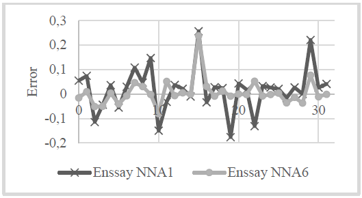
Fig. 2 describes the behavior of the root mean square errors of the NNA1 and NNA6 tests.

Source: own elaboration.
Figure 2 Behavior of the errors in the NNA1 and NNA2 tests for each circuit.
From Fig. 2 it is inferred that the error of the NNA6 network presents a more stable behavior, so based on this and the correlation coefficient obtained, it is decided to choose the NNA network as the one that best adjusts to the data involved in the study.
The behavior of the mean square error as a function of the epochs is shown in Fig. 3. Note that the validation obtained its best result in epoch two.
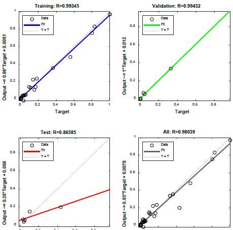
For learning the network, it chooses a set of data that is provided at each stage of learning. Fig. 4 shows the correlation coefficients obtained between the input and output variables, at each stage of network learning, belonging to the NNA6 experiment.

Source: own elaboration.
Figure 4 Correlation coefficient between input and output variables at each stage of network learning for the NNA6 experiment.
Finally, it is established that the network adjusts to the information provided with a correlation coefficient of 0.980 and a mean square error of 0.0028, approximately. The established structure of the neural network is described in Fig. 5.
In this way, the network is formed with 17 neurons in the hidden layer with 4 inputs; while the output layer presents a single neuron in its corresponding output.
3.2 Simulation or testing of the neural network
After the training of the selected network based on the minimum error and the best correlation coefficient between the variables involved in the model, the circuits are tested according to the representative information for 2020. The values corresponding to this year or variables input into the simulation are shown in Table 3.
Loss results for each circuit are presented in Fig. 6, where the circuits are identified by their corresponding disconnects.
4. Conclusions
From the results obtained, experimentally, the potentiality of the proposed model in determining the losses in subtransmission networks is corroborated with a mean square error of 0.0028 and a correlation coefficient between the variables involved of 0.980.
The neural network that better adjusts to the variables implicated in this investigation is conformed by an occult layer with 17 neurons and show transference sigmoide logarithmic and a layer of linear exit.
The proposed artificial neural network model is satisfactory for evaluating technical losses in subtransmission electrical networks, and its use is fully identified with the availability of data under the conditions of the Cuban electrical system.


