


 English (pdf)
 Article in xml format
 Article references
 Send this article by e-mail
 Cited by SciELO
  Cited by Google
  Similars in
SciELO
Similars in
SciELO  Similars in Google
 Permalink
1. Introduction
Improving healthcare quality requires permanent monitoring of the processes performance and implementation of changes to benefit users. In this regard, data analysis approaches can be implemented, but this is not a simple matter from the process performance measurement in the healthcare sector. Generally, it is required to meet some assumptions and conditions. One of the most relevant data characteristics in the health sector is the high variability in the results and the sample sizes [1].
Furthermore, the application of statistical quality control tools in the analysis of healthcare processes is not yet intensive due to the following aspects [2]: (i) There is resistance to accepting that an approach to improve the quality of industrial processes can be applied to healthcare, (ii) Statistical quality control is missing from the most popular books on medical statistics, and, (iii) Statistical quality control faces fundamental assumptions about how to develop documented improvements in healthcare.
However, quality control generates application interest in medicine and healthcare. For this, the traditional concepts of quality control of industrial processes have been adapted and transformed to be useful in monitoring health processes [3].
According to [4], control charts are used widely in different sectors such as banks, hospitals, and financial services, among others. Control charts can be applied in the healthcare sector to improve outpatient care, operating room efficiency, and also to reduce unnecessary costs and length of stay. They can also contribute to the need to monitor and control healthcare performance and minimize adverse events [5].
Additionally, control charts can help stakeholders manage change in healthcare and improve patient health [6]. Control charts allow locating and identifying the root cause of process variability to eradicate or control it [7]. The causes of variability can be classified into common and special causes.
Common or random causes are inherent to the process characteristics and eliminating or reducing them depends on modifying the system. Special or assignable causes are due to situations outside the process, that is, external factors that can be identified and eliminated [8].
The main objective of control charts is to monitor and analyze the variability behavior of a process over time [9]. Depending on the type of data, control charts can be classified into two main groups: control charts for variables (continuous data) and control charts for attributes (discrete data) [10]. This paper focuses on the control charts for attributes, specifically on the p or defective ratio control chart.
The elaboration of a p-chart is based on the fulfillment of several assumptions. First, the data are assumed to have a binomial distribution with independent events having a constant underlying probability of occurrence. In addition, the mean defective proportion must be constant over time, implying that it should not vary between subgroups [11].
Overdispersed data occur when there is excessive variability within or between subgroups. Overdispersion makes it difficult to monitor processes with traditional p-charts since some subgroups are likely to be out of control when they are not (type 1 error). Overdispersed data do not satisfy the constant defectives proportion assumption and are characteristic of processes with large sample sizes.
Monitoring of overdispersed data requires a control chart that considers variation within and between subgroups. Thus, it is possible to differentiate between common and special causes of variation [12]. For example, an analysis of data on survival after coronary artery bypass grafts, emergency readmission rates, and teenage pregnancies is made in [13]. It is established that the treatment of overdispersed data leads to the conclusion that these processes are not under control using the traditional control chart approach.
In [14], control charts are used to monitor infections and mortality in surgical facilities, concluding that when dealing with large sample sizes there could be dependence between results, and new statistical methods need to be applied. Traditional control charts have limitations for analyzing infrequent events [6].
Also, in [15], a study on the number of patients seen in the first four hours in accident and emergency departments was performed. It concludes that traditional control charts lose effectiveness when dealing with overdispersed data, and a combined charting strategy should be used.
Although several previous academic works analyze the problem of overdispersed data in traditional control charts [16], the research gap on control chart applications suitable for this data characteristic remains considerable. Therefore, in this article, we analyze the monitoring of overdispersed processes in clinical laboratories and determine the most appropriate data analysis procedure and control charts.
This work constitutes an academic contribution to the processes analysis under conditions closer to reality and promotes the use of appropriate statistical tools that allow the treatment of data that do not meet the assumptions of traditional control charts.
2. Methodology
The methodology includes four steps: (i) Determination of the interest variable, (ii) Diagnosis of data overdispersion, (iii) Elaboration of control charts, and (iv) Analysis of results.
2.1. Determination of the interest variable
The sample processing in clinical laboratories requires adequate sample collection for the following tests and avoiding false negatives and false positives in the results. When the sample does not meet the established requirements, it is discarded and becomes a defective product from the perspective of statistical quality control.
Discarded samples generate waste of clinical laboratory resources and can cause user dissatisfaction because a new sampling is required. Therefore, it is essential to implement programs to monitor and control the sampling effectiveness to prevent errors in clinical tests and make decisions to improve the health service.
The data of this article are from a clinical laboratory in Colombia, with continuous monitoring for one year. The interesting variable is the number of clinical samples discarded per week, with a total monitoring time of 50 weeks. Thus, the monitoring parameter (p) in the control charts is the proportion of samples discarded in each subgroup (week).
2.2. Diagnosis of data overdispersion
The diagnosis of process data overdispersion is performed using the Jones and Govindaraju [17] and Heimann [18] methods.
Jones and Govindaraju [17] proposed a graphical method based on the variance ratio test (VRT), comparing the observed variation in a data sample and the expected variation of the corresponding binomial distribution. Let d i be considered a number of nonconforming units in i subgroups of size n that follow a binomial distribution with parameter p (proportion of the nonconforming units), then:

follows a normal distribution with mean
 and variance
 :
:
where
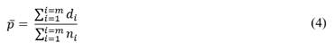
The procedure of this method begins by transforming data using (1) and then constructing the normal probability plot of the transformed data and its fitting line. Subsequently, the actual variation of the process is estimated as the distance on the y i axis that intercepts with the scores +1 y -1 of Z in the fitting line. If the actual variation is greater than the expected variation, estimated as 1.5/√n, it is concluded that the data are overdispersed and it is not possible to state that they follow a binomial distribution.
On the other hand, Heimann [18] proposes a method based on decomposing the total variance and its representation as the sum of the sampling variance and the process variance. The sampling variance represents the difference between the estimate of the probability of producing nonconforming units (from the sample) and the actual value (from the process). The underlying process variance represents the variation in the probability of producing nonconforming units.
Thus, the sampling variance
 is determined by:

Similarly, let  is determined as follows:

and the underlying process variance
 results from:

Then, r is defined as the variance ratio, between the total variance and the sampling variance:

If r > 1.357, it is concluded that there is extra variability in the data, greater than a binomial distribution implies, and it is not appropriate to choose a p-chart for process monitoring and control.
2.3. Elaboration of control charts
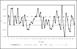
Various control chart types are developed and compared in order to select the most suitable one for monitoring overdispersed processes in clinical laboratories. Therefore, we develop the p-chart with variable limits, normalized p-chart (Z), moving range chart (X-MR), p’-chart of Laney, and the chart proposed by Goedhart and Woodall.
The construction procedures of the first three control charts are not described in this article since they are widely known and extensively detailed in textbooks on statistical quality control [10] [19]. The construction procedures for the last two control charts are detailed below.
2.3.1. p´-chart of Laney
This control chart considers both intra-sample and inter-sample variation, with a multiplicative effect for calculating the control limits (CLs) [11]:

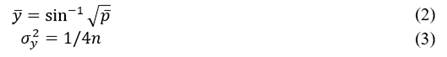
Where σz is the inter-sample variation and σ pi is the intra-sample variation:
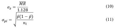
where  is the average proportion, and
 is the average moving range of the z-scores for each subgroup, z
i
:
is the average moving range of the z-scores for each subgroup, z
i
:

2.3.2. p-chart of Goedhart and Woodall
In this control chart, the control limits (CLs) are calculated based on an adding ratio of the intra-sample and inter-sample variations, considering the average standard deviation of the proportion
 [20]:
[20]:

where
 is the intra-sample variance,
 is the inter-sample variance and
3. Results
3.1. Data description of the interest variable
Table 1 shows the data collected from monitoring the total number of samples collected and the number of samples discarded per week in the clinical laboratory under study. The average proportion of nonconforming units,
 is equal to 0.05. This relatively low value, regarding the standards set by the laboratory, could lead to preliminary inferences that the process has large sample sizes or a low number of nonconforming units per subgroup.
Table 1 Total samples and Nonconforming samples per week.
| Week | Total samples | Nonconforming Samples | Week | Total samples | Nonconforming Samples |
|---|---|---|---|---|---|
| 1 | 1467 | 105 | 26 | 1591 | 34 |
| 2 | 1789 | 68 | 27 | 1726 | 112 |
| 3 | 1345 | 140 | 28 | 1279 | 25 |
| 4 | 2347 | 217 | 29 | 2430 | 132 |
| 5 | 1734 | 61 | 30 | 275 | 6 |
| 6 | 2378 | 158 | 31 | 1784 | 96 |
| 7 | 1893 | 80 | 32 | 2694 | 74 |
| 8 | 2992 | 260 | 33 | 3583 | 101 |
| 9 | 1935 | 81 | 34 | 6945 | 276 |
| 10 | 1967 | 87 | 35 | 2895 | 184 |
| 11 | 1524 | 98 | 36 | 7492 | 351 |
| 12 | 2592 | 91 | 37 | 1764 | 155 |
| 13 | 3890 | 254 | 38 | 3790 | 226 |
| 14 | 1469 | 79 | 39 | 2578 | 101 |
| 15 | 2693 | 67 | 40 | 3895 | 114 |
| 16 | 2936 | 72 | 41 | 4895 | 415 |
| 17 | 1798 | 66 | 42 | 2654 | 78 |
| 18 | 2348 | 109 | 43 | 4569 | 62 |
| 19 | 1633 | 67 | 44 | 2697 | 200 |
| 20 | 1376 | 80 | 45 | 2589 | 143 |
| 21 | 1234 | 88 | 46 | 2478 | 62 |
| 22 | 1357 | 98 | 47 | 2737 | 49 |
| 23 | 1594 | 158 | 48 | 1839 | 129 |
| 24 | 3789 | 238 | 49 | 1426 | 84 |
| 25 | 1598 | 135 | 50 | 1925 | 75 |
| TOTAL | 124208 | 6241 |
Source: The authors.
Table 1 shows that both the sample sizes and the number of nonconforming units per subgroup have a high variation. However, the average sample variance is 0.00002559, a relatively low value. This requires a detailed analysis of the data dispersion, as detailed in the next step.
3.2. Results of data overdispersion diagnosis
Fig. 1 shows the normal probability plot of the data transformed by applying the Jones and Govindaraju method, described in section 2.2. According to the results, the actual process variation is equal to 0.1073 and the expected variation is equal to 0.0905. Since the actual variance is greater than the expected variance, it is possible to state that the process data are overdispersed.

Moreover, applying the Heimann method, it is obtained that
 = 0.000026 and
 = 0.000537. Therefore, the variance ratio r is equal to 20.65. Since r > 1.357, it can be stated that the data have a higher variation than expected for a binomial distribution.
Finally, it is possible to state that the highest variation corresponds to the underlying process variation. Data overdispersion is identified in both diagnostic methods, therefore, it is not appropriate to choose a traditional p-chart for process monitoring and control.
3.3 Elaboration of control charts
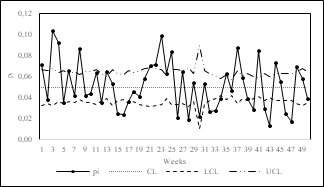
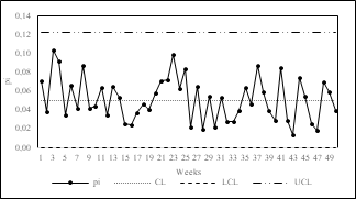
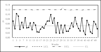
In order to compare performance and select the most appropriate control chart(s) for monitoring overdispersed processes in clinical laboratories, we developed the p-chart with variable limits (Fig. 2), the normalized p-chart (Fig. 3), X-MR chart (Fig. 4), p’-chart of Laney (Fig. 5) and the p-chart of Goedhart and Woodall (Fig. 6). The control charts were made using Microsoft Excel©.

3.4. Analysis of results
Traditional control charts have limitations for monitoring overdispersed data due to the assumptions required for their construction [21]. The p-chart with variable limits and the normalized p-chart assume a binomial distribution of the data and that the mean remains constant over time.
The above two assumptions are not satisfied in overdispersed data. Therefore, many points fall outside the control limits, as shown in Figs. 2 and 3. Because of that, it is not appropriate to use either of these two control charts for monitoring overdispersed processes since the data assumptions are not satisfied, and type 1 errors may occur.
According to [17], the acceptable solution for decades to monitor overdispersed data was the development of the X-MR chart (Fig. 4). Although this control chart also assumes a binomial distribution of the data, it incorporates compensation for the inter-sample variation by considering the average moving range as a factor for calculating the control limits. However, it does not consider inter-sample variation and presents constant control limits.
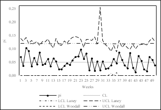
The p'-chart of Laney (Fig. 5) and the p-chart of Goedhart and Woodall (Fig. 6) overcome the limitations of previous control charts and have variable control limits that adjust depending on inter-sample and intra-sample variation. As mentioned in section 2.3, the main difference between these two control charts lies in the effect of inter-sample and intra-sample variations in calculating the control limits. While the p'-chart of Laney has a multiplicative approach, the p-chart of Goedhart and Woodall has an additive approach.
The latter is shown in Fig. 7. The multiplicative effect of the variances causes higher variability in the width of the control limits in the Laney control chart. The maximum range of variation of the control limits, obtained as the difference between the extreme values of the control limits in each control chart, is higher in the p'-chart of Laney (0.255) than in the p-chart of Goedhart and Woodall (0.129). The p-chart of Goedhart and Woodall has control limits that do not overestimate the effect of variances and therefore have lower variability over time.
Finally, Table 2 shows a comparative summary of the control charts analyzed based on the results of this work. The decision on the control chart adequate to monitor overdispersed processes depends on fulfilling two main conditions: (i) The control chart must be applicable without data distributional, and stability of the process mean assumptions, and (ii) The control chart must consider both intra-sample and inter-sample variances.
Table 2 Comparative overview of control charts for monitoring overdispersed processes.
| Control chart | Applicable without data distributional assumptions? | Consider both intra-sample and inter-sample variances? | Adequate for overdispersed data monitoring? |
|---|---|---|---|
| p-chart | No | No | No |
| Z-chart | No | No | No |
| X-MR chart | No | No | No |
| p´-Laney | Yes | Yes | Yes |
| p-Goedhart & Woodall | Yes | Yes | Yes |
Source: The authors.
4. Conclusions
Monitoring the proportion of nonconforming units in clinical laboratories is important for quality assurance in patient service and proper process management. Process data in clinical laboratories present high variability because the number of samples taken varies over time since it depends on patient demand. Human intervention in sample collection and processing also increases the variability of the results.
Excessive variability in clinical processes means that the data are overdispersed and do not fulfill the assumptions required for monitoring using traditional control charts. In these cases, using control charts can lead to erroneous conclusions about the process behavior. For this reason, it is necessary to develop comprehensive studies that consider the data characteristics for implementing quality control tools in the health sector.
In this paper, we performed a comparative study of the application of different control charts for monitoring overdispersed processes in clinical laboratories. We also proposed a methodological scheme for adequate monitoring, focused on the diagnosis of data overdispersion through a graphical and an analytical method.
The proposed methodological approach and the developed case study led to conclude that the main criterion for applying control charts in overdispersed processes is to consider both the inter-sample and intra-sample variations and their effect on the calculation of the control limits.
This article is a product of ongoing research whose main objective is to improve statistical process management programs in the health sector. The following research stage will apply the methodology considering other attributes such as non-conformities.
It is also of interest to make applications in areas such as patient care in hospitals, monitoring of drug prescriptions, climatic or environmental phenomena, and, overall, processes where the sample size has a high variability between batches.

