


 English (pdf)
 Article in xml format
 Article references
 Send this article by e-mail
 Cited by SciELO
  Cited by Google
  Similars in
SciELO
Similars in
SciELO  Similars in Google
 Permalink
1. Introduction
The usual methodology of bridge design processes is a "trial and error" procedure. The designer proposes initial dimensions based on his experience, and from there begins a simple iterative process until the structure meets the design criteria. However, these designs are usually irrational due to the large number of variables involved in these problems. If we add the fact that in developing regions there are no up-to-date and reliable databases on the real costs (economic, environmental, etc.) of building materials and activities [1], obviously the design recommendations used by the designer are often not the right ones. That is why in recent years there has been a great thriving in a science named Structural Optimization, by means of which all the variables that affect the problem in question can be taken into account, providing much more rational solutions than those obtained by the traditional method.
Many authors have been dedicated to the development and application of bridge design optimization methodologies. [2] present the minimum cost automatic design of precast bridge decks made of U-beams and upper deck. An optimal memetic algorithm is used, and as a result, between 8 and 50% economic savings are obtained with respect to structures already built. In [3] the multi-objective optimization of the design of post-tensioned concrete box-girder road bridges is performed, taking into account the economic criteria, CO2 emissions and global safety factor. The multi-objective Harmony Search method is used. Here it is identified that the economic and environmental optimization are closely related, i.e., they provide similar results. In addition, a series of recommendations are provided based on the results obtained for each objective. In [4] a similar work is performed, additionally adding durability criteria, measured by the corrosion initiation time. Furthermore, Neural Networks are used to accelerate the convergence processes of these procedures, which are generally quite expensive [1,5,6]. In [7] the concept of Reliability-Based Design is also introduced in these problems. For their part, [8] use the Simulated Annealing algorithm for the design optimization of prestressed concrete slab bridge decks, where an analysis is made of the solutions obtained including other environmental criteria such as Embodied Energy, and their differences with the economic optimization. As can be seen, in all these works, the case studies are made of prestressed or post-tensioned concrete, which is the recommended solution for bridges with long spans. However, in Cuba, the steel used for these solutions is imported and holds a high economic cost. In the thesis [9] the design of the superstructure of prestressed concrete road bridges is optimized, where the solutions tend to elements with large cross sectional elements, in order to avoid the use of prestressing steel. Therefore, this work proposes the alternative of using reinforced concrete (RC) as the most rational solution, from the economic point of view.
The structure of the paper is as follows. Section 2 is used to explain the proposed methodology, including the mathematical formulation of the optimization problem, a brief description of the case study, and the introduction of the BBO method. In section 3, we discuss the obtained results and comparisons between optimized and traditional designs are made.
2. Materials and methods
2.1. Optimization problem definition
In this work, the complete formulation of the structural optimization problem for three-span reinforced concrete beam-deck type road bridges is elaborated. Starting from a pre-dimensioning, the structure and load system of a bridge type is modeled, the variables and constraints are defined, and the objective function is declared under the criterion of minimization of the direct construction cost.
2.1.1. General description and modeling of the structure
The case studies will be focused on covering spans of 40, 50 and 60 m, with two solutions for each span to be covered. Therefore, there will be six case studies, and thus, in addition to obtaining the best solution for each independent configuration, a general recommendation will be obtained on how to distribute the sub-spans according to the general span to be covered. This distribution is shown in Table 1.
Table 1 Span combinations for case studies.
| Configuration | Extreme Span (m) | Central Span (m) | Extreme Span (m) | Bridge length (m) |
|---|---|---|---|---|
| 1 | 12 | 16 | 12 | 40 |
| 2 | 10 | 20 | 10 | 40 |
| 3 | 16 | 18 | 16 | 50 |
| 4 | 14 | 22 | 14 | 50 |
| 5 | 18 | 24 | 18 | 60 |
| 6 | 16 | 28 | 16 | 60 |
Source: The Authors
The bridges correspond to Category I roads, with traffic intensity (PAVDT) between 4000 and 8000 vehicles/day. The roadway is composed of two 3.75 m wide traffic lanes, with 3.00 m wide walkways on both sides of the road, complying with the specifications of [10]. A flexible pavement thickness of 8 cm is established, consisting of a 5 cm layer of semi-dense asphalt concrete and a 3 cm layer of dense asphalt concrete. Sidewalks are not contemplated for the case study, but concrete railings of 0.75 m in height above the level of the roadway will be included.
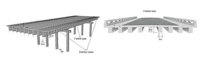
Bridges models will be hyper-static, with 3 spans, beam type and RC deck (see Fig. 1). The beams will be precast ones with rectangular cross-section, continuous along the length of the bridge. Continuity will be achieved by means of steel protruding from the longitudinal reinforcement, which will be spliced to the next girder, re-casting the formed joint with in-situ concrete. The beams are supported on RC pier caps of rectangular section, and these on 4 columns of square section also made of RC. For this study no diaphragms are considered, and the foundation and abutments are excluded from the analysis, modeling the link of the latter as elastic neoprene supports with finite stiffness.
Permanent actions are considered to be the self-weight of each of the elements of the assembly (DC) and the self-weight of the bearing surfaces and utility installations (DW). As transitory actions, the design vehicular overload (LL) on bridge roadways and the longitudinal action due to braking or starting of vehicles (BR) according to [11] are considered. As a temporary action, the wind incidence (WS) is also analyzed, calculated according to [12], which takes into account the horizontal and vertical wind load applied on the deck surface, the wind load applied to columns, the leeward beam and the windward beam. In general, it is taken into account 38 load combinations grouped into: Resistance I, Resistance III, Resistance IV, Resistance V, Serviceability and Serviceability of Permanent Loads, according to the AASHTO standard [11].
Bridge dimensions and loads are modeled in CSiBridge© [13]. A linear analysis by finite elements is carried out. CSiBridge© is linked with Matlab© to create the model with the bridge information and to extract the results of the structural analysis and design. CSiBridge© has an Open Application Programming Interface (OAPI) to allow other software to be integrated with it.
CSiBridge© is used for the finite-element analysis. Matlab© is used to control the finite-element analysis, check the limit states and evaluate the objective functions.
2.1.2. Objective function
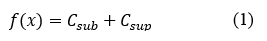
Since the optimization criterion selected for this research is the minimum total cost, the objective function, represented in Eq. (1), is defined as the sum of the direct construction costs of the substructure and superstructure.
The cost of the substructure is composed of the sum of the direct costs of earthworks, foundations, columns and pier caps. The cost of the superstructure contains the direct cost of the beams, deck, walks, wearing course and defenses. The cost of earthwork and foundations was calculated based on technical-economic indicators. The rest of the costs are calculated using unit prices obtained from [14] and are shown in Table 2. In the case of steel and concrete, the cost of elaboration, assembly (for steel) and placement are taken into account.
Table 2 Unit costs used to calculate direct construction costs.
| Item | Direct Cost per unit (Cuban Pesos) |
|---|---|
| m² of formwork in columns | 13.14 |
| m² of formwork in beams and pier caps | 11.57 |
| m² of formwork in deck | 8.96 |
| Kg of steel in columns | 453.74 |
| Kg of steel in beams and pier caps | 453.74 |
| Kg of steel in deck | 432.81 |
| m³ concrete 25 MPa (material) | 49.06 |
| m³ concrete 30 Mpa (material) | 52.27 |
| m³ concrete 35 Mpa (material) | 55.04 |
| m³ concrete 40 Mpa (material) | 68.99 |
| Placement of m³ of concrete in columns | 9.4 |
| Placement of m³ of concrete in beams and pier caps | 9.4 |
| Placement of m³ of concrete in deck | 3.14 |
Source: The Authors
2.1.3. Variables
The variables are discrete, since structural optimization demands final solutions that are constructively feasible, in addition to significantly reducing the solution space. For these case studies, there are 11 independent variables shown in Fig. 1 and Table 3: (x1) number of girders (beams) in the bridge cross section, (x2) thickness of the top deck, (x3) bridge center span girder depth, (x4) bridge center span girder width, (x5) bridge extreme spans girder depth, (x6) bridge extreme spans girder width, (x7) columns depth, (x8) girder concrete quality, (x9) deck concrete quality, (x10) column concrete quality, and (x11) pier cap concrete quality. The following are defined as dependent variables: the depth and width of the pier caps (sized according to the depth of the columns), the longitudinal and transversal steel areas of beams, deck, pier caps and columns, obtained once the design is carried out.
Table 3 Independent variables and their movement intervals
| Variable | Range | u/m |
|---|---|---|
| Number of girders (beams) (nv) | 5 ≤ x1 ≤ 11 | u |
| Deck thickness (t) | 0.16 ≤ x2 ≤ 0.26 | m |
| Central beams depth (hvc) | 1.05 ≤ x3 ≤ 2.45 | m |
| Central beams width (bvc) | 0.45 ≤ x4 ≤ 0.95 | m |
| Extreme beams depth (hve) | 0.4 ≤ x5 ≤ 1.45 | m |
| Extreme beams width (bve) | 0.15 ≤ x6 ≤ 0.65 | m |
| Columns depth (hp) | 0.50 ≤ x7 ≤ 1.00 | m |
| 𝑓′𝑐 beams | 25 ≤ x8≤ 40 | MPa |
| 𝑓′𝑐 deck | 25 ≤ x9 ≤ 40 | MPa |
| 𝑓′𝑐 columns | 25 ≤ x10 ≤ 40 | MPa |
| 𝑓′𝑐 pier caps | 25 ≤ x11 ≤ 40 | MPa |
Source: The Authors
2.1.4. Constraints
The fulfillment of the constraints ensures that the bridge, as a result of the solution of the optimization problem, is constructible because it makes physical sense and meets the structural safety requirements. Constraints can be divided in two types: implicit and explicit.
The implicit ones are mainly associated with the fulfillment of the conditions imposed by the design (state equations) through the limit states (strength, stiffness) and they are introduced in the proposed solution algorithm [1,5,6]. The resistance conditions are met when performing the design of the elements, either in those that are designed by the CSI Bridge itself (columns and pier caps) using the AASHTO LRFD-2014 code, or in those that are designed using a routine programmed in MATLAB (beams and deck) based on the specifications of the Cuban standard [15]. The deflection of the elements subjected to bending and crack openings are checked within the design routine itself, where the objective function is penalized, in case of non-compliance. Within the algorithm, other constructive constraints are also established, such as those related to the placement of longitudinal and transversal steel in beams, columns and pier caps.
The explicit constraints limit the range of movement of the variables in the optimization process (minimum and maximum limits they can take), a mandatory requirement of the methods used in this research.
2.2. Modeling, analysis and structural design of the bridge
The modeling of the study bridges was performed in CSIBridge20. As permanent actions, the self-weight of each of the elements is considered, which is automatically calculated by CSIBridge20 from the dimensions and volumetric weights of the component materials, the self-weight of the bearing surfaces (1.84 kN/m²) and the load transmitted by the guardrails or fenders on both sides of the road (2.95 kN/m).
As transitory actions, the braking load and vehicular overload are taken into account according to [11], the latter represented by the HL-93 vehicle, which combines the action of the design truck or design tandem and the rail load. In addition, the wind load is taken into account according to the specifications of the Cuban standard [12]. The study takes into account 38 load combinations grouped into: Resistance I, Resistance III, Resistance IV, Resistance V, Service and Permanent Load Service. The load factors were assigned according to the AASHTO standard.
The structural design of the beams and the deck is performed by means of a routine programmed in MATLAB based on the specifications of the Cuban standard [15]. The total deflection in both elements is also determined, which is then compared with the allowable deflection. Compliance with the allowable crack opening is ensured during design by controlling that the separation between reinforcement bars does not exceed the maximum allowable by-standards separation.
2.3. Biogeography-Based Optimization
Biogeography studies the geographical distribution of biological organisms. Mathematical models of biogeography describe how species migrate from one habitat or island to another, how new species arise, and how species become extinct. Geographical areas that are well suited as residences for biological species are said to have a high habitat suitability index (HSI). Habitats with a high HSI have a high species emigration rate, because they host many species able to emigrate to neighboring habitats, and they have a low species immigration rate because they are already nearly saturated with species. Therefore, high HSI habitats are more static in their species distribution than low HSI habitats. Habitats with a low HSI have a high species immigration rate because of their sparse populations. This immigration may raise the HSI of the habitat, because the suitability of a habitat is proportional to its biological diversity. However, if a habitat’s HSI remains low, the residing species tend to go extinct, which will further open the way for additional immigration. Due to this, low HSI habitats are more dynamic in their species distribution than high HSI habitats [6,16].
The Biogeography-Based Optimization (BBO) method, proposed in Simon (2008), is a relatively new method based on the concepts explained above. The correspondence between the BBO population, individuals (solutions), gens and fitness value. Hence, the number of species in each habitat is equal to the number of variables in the optimization problem [1,6]. The algorithm consists of the following steps:
The algorithm starts with a random initial set of habitats with a uniform HIS distribution.
In every iteration, the emigration and immigration coefficients, denoted by respectively μ and λ, are assigned to each habitat. Solutions or habitats with a high HSI receive high values of μ and low values of λ, and vice versa.
The algorithm processes the habitats in order of decreasing HSI, using the parameters μ, λ and mutation probability as follows:
Within each habitat, for each species the possibility to carry out the migration process is analyzed: each species is checked based on the habitat’s immigration coefficient λ. Therefore, the species of the best habitats have little chance of entering this process, while this chance increases when considering habitats with a higher λ.
Once a species enters the migration process, another species from other habitat is selected using roulette wheel selection (to select the habitat) based on μ to immigrate to the habitat being worked on.
Once the species are selected, immigration starts, which is not the substitution of one by the other, but a combination of both, performed as:

where Species i k , i.e. the k-th species of habitat i, is the species being analyzed and Species j k , i.e. the k-th species of habitat j, is the species selected to immigrate, and α is the acceleration coefficient (0.9 per default).
- In addition, species can mutate with a certain probability according to:
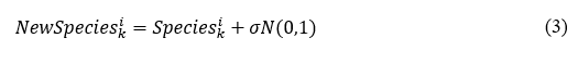
where σ is the mutation step size (0.05 per default), N(0,1) is a random number with mean 0 and standard deviation 1. After every iteration, σ decreases, modified by the mutation step size damping (0.99 per default).
4. Once the entire population is analyzed, the new one is formed by selecting the best habitats of the previous population (before being transformed) and the best of the new population. The fraction of the previous population that survives is denoted by KeepRate. This is similar to elitism used in GA. This iterative process ends when a stop criterion is satisfied.
2.4. General algorithm
The entire procedure is programmed in Matlab©, using CSiBridge© as the calculation engine through the API functions. In general, the algorithm consists of the following general steps (see Fig. 2):
Decoding the vector containing the set of design variables.
Starting CSIBridge20 and loading the model
Assigning properties and dimensions to the elements
Adding load patterns
Executing the analysis
Design of deck, columns, pier cab and beams
Calculation of the Budget
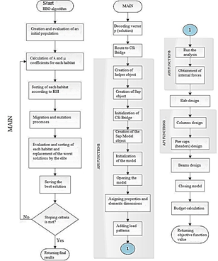
3. Results and discussion
The results will be divided as follows: first, a small sensitivity analysis of the BBO parameters for this type of problem is performed, the optimal designs obtained and the influence of each of the variables on these results are presented, and finally, an analysis of the differences in the results obtained with respect to the traditional designs is made.
3.1. Sensitivity analysis of BBO parameters
These configurations have not been chosen arbitrarily. Process # 1 is based on the results of BBO parameter tuning in the optimization of RC structures [5,6]. Process # 2 involves the parameter configuration that proved to be the most effective in a work on optimal sensor placement, which is ongoing. Process # 3 consists of a variation of the number of iterations of the first one, assuming that the number of max iterations established could not be enough. The two reference works are completely different, although they have the particularity of being applications of BBO to discrete optimization.
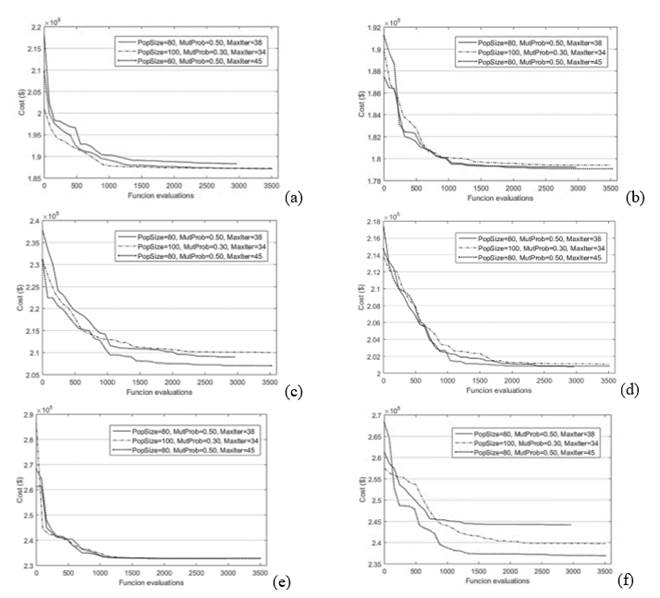
Fig. 3 shows how the third configuration (PopSize=80, MutProb=0.50 and MaxIter=45) is the best option, although in general terms, the differences are not so significant, demonstrating that BBO is a great generalist, i.e., that it offers good performance regardless its parameter configuration.
Source: The Authors
Figure 3 Average performance curves (fitness value in function of the function evaluations) of five optimization process for each model, (a) and (b) correspond to 40 m bridge (10-20-10 and 12-16-12 respectively), (c) and (d) correspond to 50 m bridge (14-22-14 and 16-18-16 respectively) and (e) and (f) correspond to 60 m bridge (16-28-16 and 18-24-18 respectively).
3.2. Optimal designs and influence of variables
Table 4 shows the value of the best solution for each model. It can be seen how the configurations showing a more equal distribution between the extreme and center spans generally offer a better and more economical solution.
Table 4 Results obtained for each configuration.
| Models | Minimum direct cost ($) |
|---|---|
| 40 m: 10-20-10 | 184,353.69 |
| 40 m: 12-16-12 | 178,605.24 |
| 50 m: 14-22-14 | 205,568.57 |
| 50 m: 16-18-16 | 200,662.31 |
| 60 m: 16-28-16 | 232,735.82 |
| 60 m: 18-24-18 | 234,355.55 |
Source: The Authors
Table 5 shows the results for the variable "number of beams" and those related to the deck. In addition, the top and bottom reinforcement ratios in decks are shown. Here it can be seen that a common feature is the selection of few beams as the most economical option, although this implies an increase in deck thickness. The optimum concrete quality for the deck is common for all variants. This is the logical value since it is an element that works mostly in bending, so the compressive strength of the concrete is not a determining factor. The most common reinforcement ratios are 0.65% for top longitudinal reinforcement and 0.10 to 0.12% for bottom longitudinal reinforcement. For both top and bottom transversal reinforcement, it ranges from 1.01 to 1.33%.
Table 5 Results related to number of beams and deck configuration.
| Models | Number of beams (u) | Deck thickness (m) | Deck concrete quality (MPa) | Deck reinf. ratio | |||
|---|---|---|---|---|---|---|---|
| Long. Reinf. (%) | Trans. Reinf. (%) | ||||||
| (+ | (- | (+ | (- | ||||
| 40 m: 10-20-10 | 5 | 0.24 | 25 | 0.65 | 0.10 | 1.01 | 1.01 |
| 40 m: 12-16-12 | 5 | 0.24 | 25 | 0.65 | 0.10 | 1.01 | 1.01 |
| 50 m: 14-22-14 | 5 | 0.24 | 25 | 0.65 | 0.10 | 1.01 | 1.01 |
| 50 m: 16-18-16 | 7 | 0.16 | 25 | 0.92 | 0.21 | 1.76 | 0.21 |
| 60 m: 16-28-16 | 5 | 0.22 | 25 | 0.65 | 0.12 | 1.33 | 1.33 |
| 60 m: 18-24-18 | 5 | 0.22 | 25 | 0.65 | 0.12 | 1.33 | 1.33 |
Source: The Authors
Table 6 shows the results related to the beams. It can be seen how the fact of decreasing the number of beams leads to large depths due to the increase in the interior forces that each beam must resist individually.
Table 6 Results related to beams.
| Models | Central beams depth (m) | Central beams width (m) | Extreme beams depth (m) | Extreme beams width (m) | Conc. quality (MPa) |
|---|---|---|---|---|---|
| 40 m: 10-20-10 | 1.80 | 0.45 | 0.75 | 0.45 | 35 |
| 40 m: 12-16-12 | 1.40 | 0.35 | 0.90 | 0.45 | 25 |
| 50 m: 14-22-14 | 1.95 | 0.50 | 0.90 | 0.55 | 25 |
| 50 m: 16-18-16 | 1.25 | 0.40 | 1.20 | 0.40 | 35 |
| 60 m: 16-28-16 | 1.95 | 0.65 | 1.25 | 0.45 | 35 |
| 60 m: 18-24-18 | 1.95 | 0.55 | 1.15 | 0.60 | 25 |
Source: The Authors
In addition, it is observed that the rectangularity of the beams presents values between 3 and 4 for the central beams, and from 1.6 to 3 for the exterior ones, which shows a predisposition to slender elements. On the other hand, unlike the deck, the beams, although they work in bending, show a certain tendency to increase the quality of the concrete. This is due to the fact that, as mentioned above, these elements have large depths, so that the concrete compression block is much more significant than in the case of the deck, increasing the influence of the concrete quality on the flexural resistance of beams.
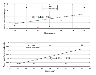
Fig. 4 shows the variation of the optimum depths of the beams as a function of their span. It also shows the fitted curve according to the points obtained for each case. Fig. 5 shows more specific results, since the beams of the central and extreme spans are divided. The beam depth/beam Span ratio is an aspect usually used by researchers and designers as design recommendations for classic design procedures.

Source: The Authors
Figure 5 Beam Span/Beam depth ratio in function of beam span for (a) central and (b) extreme beams
Another aspect usually provided as a design recommendation is the reinforcement ratio for beams. It gives an idea of how the steel/concrete ratio should behave in order to achieve efficient designs. Table 7 shows the most representative values for this aspect. The maximum amounts of top reinforcement in the central beams range from 1.01 to 1.46%, while those of bottom reinforcement range from 0.66 to 1.11%. For the extreme beams, maximum values of 0.96 to 1.33% for the top reinforcement and 1.90 to 2.35% for the bottom reinforcement are obtained. Summarizing, optimal reinforcement ratios represent 44 to 53% of the balanced one.
Table 7 Optimal reinforcement ratios in beams
| Models | Interior beam-extreme Span | Interior beam-central Span | Exterior beam-extreme Span | Exterior beam-extreme Span | ||||
|---|---|---|---|---|---|---|---|---|
| (+ (%) | (- (%) | (+ (%) | (- (%) | (+ (%) | (- (%) | (+ (%) | (- (%) | |
| 40 m: 10-20-10 | 1.01 | 0.51 | 1.27 | 0.51 | 0.96 | 1.61 | 0.54 | 2.35 |
| 40 m: 12-16-12 | 0.99 | 0.61 | 1.46 | 1.11 | 0.93 | 1.06 | 0.52 | 2.12 |
| 50 m: 14-22-14 | 0.96 | 0.48 | 1.04 | 0.48 | 0.93 | 1.90 | 0.48 | 1.90 |
| 50 m: 16-18-16 | 0.97 | 0.66 | 1.28 | 1.09 | 0.75 | 0.97 | 1.33 | 1.48 |
| 60 m: 16-28-16 | 0.99 | 0.51 | 0.99 | 0.51 | 0.69 | 0.98 | 1.19 | 1.63 |
| 60 m: 18-24-18 | 0.95 | 0.52 | 0.95 | 0.80 | 0.93 | 1.55 | 0.47 | 1.51 |
Source: The Authors
On the other hand, the dimensions of columns and piers do not vary greatly from one model to another (Table 8). Pile depths are close to the lower limit of the literature recommendations (0.5 to 0.9 m). The quality of the concrete in the columns is equal or superior to 30 MPa, and in the piers between 25 and 30 MPa, both criteria being in correspondence with the nature of the behavior of each element.
Table 8 Optimal values for columns and pier caps
| Models | Col. depth (m) | Concrete quality in col. (MPa) | Reinf. Ratio in col. ( (%) | Pier width 1 (m) | Pier depth 1 (m) | Concrete quality in piers (MPa) |
|---|---|---|---|---|---|---|
| 40 m: 10-20-10 | 0.50 | 40 | 3.2% | 0.60 | 0.75 | 25 |
| 40 m: 12-16-12 | 0.60 | 30 | 1.4% | 0.70 | 0.85 | 30 |
| 50 m: 14-22-14 | 0.60 | 30 | 1.3% | 0.70 | 0.85 | 30 |
| 50 m: 16-18-16 | 0.60 | 35 | 1.3% | 0.70 | 0.85 | 30 |
| 60 m: 16-28-16 | 0.60 | 35 | 1.1% | 0.70 | 0.85 | 30 |
| 60 m: 18-24-18 | 0.70 | 25 | 1.0% | 0.80 | 0.95 | 25 |
| 1The width and depth of the pier are calculated as a function of the depth of the columns, so they are dependent variables of the problem. | ||||||
Source: The Authors
3.3. Differences between optimized and conventional designs
This section provides the main differences of the optimized models with the typical projects used in Cuba. Table 9 compares the total direct cost of three types of projects currently in use with the proposed variants and their corresponding design when applying the optimization algorithm. Since only one variant of the typical project coincides exactly in length with the optimized bridges, the direct cost per linear meter of bridge (Direct cost/lm) is considered as a reference for the comparison.
Table 9 Comparison of direct costs of optimized models with conventional projects
| Conventional projects | Optimized design | |||
|---|---|---|---|---|
| Variant | Direct cost/lm ($/lm) | Model | Direct cost/lm ($/lm) | Ratio of conventional project cost to optimized design |
| 40 m 12-16-12 Hiperestatic1 | 1,722.43 | 40 m: 10-20-10 | 1736.67 | 0.99 |
| 40 m: 12-16-12 | 1592.96 | 1.08 | ||
| 48 m 14-20-14 Hiperestatic1 | 1,869.72 | 50 m: 14-22-14 | 1813.64 | 1.03 |
| 50 m: 16-18-16 | 1715.51 | 1.09 | ||
| 60 m (Modified) 20-20-20 Isostatic 2 | 2,385.78 | 60 m: 16-28-16 | 1964.15 | 1.21 |
| 60 m: 18-24-18 | 1991.15 | 1.20 | ||
|
1 Typical Cuban-Soviet project 2 Variant of RC bridge project for the Caibarién - Cayo Santa María causeway | ||||
Source: The Authors
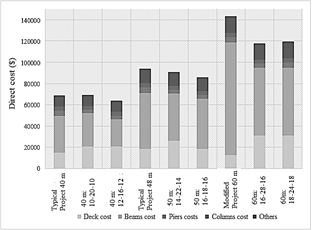
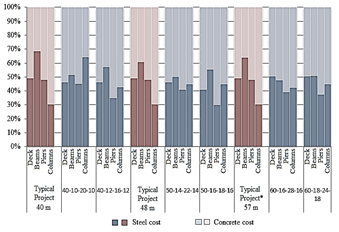
Here it can be seen that by applying the proposed algorithm, considerable savings are obtained: 8, 9 and 21 % for the combinations of 40, 50 and 60 m respectively. With the support of Fig. 6, it is possible to extract data that justify these results. Obviously, the most significant one is the reduction in the cost of the beams, produced by the reduction in the number of them. This means beams of larger dimensions, increasing the ratio of concrete to reinforcing steel, i.e., with this configuration, larger elements are obtained, reducing the need to use so much reinforcement. Fig. 7 supports this fact, as it can be seen that the optimized designs tend to "balance" the costs of concrete and steel, not only in the beams, but in all the elements. This is curious since, even though in Cuba ordinary steel is relatively cheap with respect to concrete, the traditional designs hold an excess of reinforcing steel, due to the use of many beams in the superstructure configuration, opposed to the solutions proposed by the optimization algorithm. Table 10 shows the steel to concrete ratios for typical projects and optimized designs. Here it can be seen how, to balance the steel and concrete costs, about 140 kg of steel per m3 of concrete should be used (steel/concrete cost ratio about 1.00), as opposed to about 170 used in typical projects (steel/concrete cost ratio of 1.25-1.40).
Source: The Authors
Figure 6 Breakdown of total direct cost in components (deck, beams, piers, columns and others) for each configuration.
*This typical project is not the same one shown in figure 6 (the modified) Source: The Authors
Figure 7 Percentage of costs steel/concrete for elements of each configuration.
Table 10 Steel-to-concrete amount and cost ratios for typical project and optimal designs.
| Typical Cuban-Soviet Project | Optimized design | ||||
|---|---|---|---|---|---|
| Bridge length | Kg of steel per m³ of concrete | Ratio of steel cost to concrete cost | Model | Kg of steel per m³ of concrete | Ratio of steel cost to concrete cost |
| 40 m | 185.73 kg/m³ | 1.42 | 40 m 10-20-10 | 146.43 kg/m³ | 0.99 |
| 40 m 12-16-12 | 147.53 kg/m³ | 1.00 | |||
| 48 m | 163.66 kg/m³ | 1.25 | 50 m 14-22-14 | 136.54 kg/m³ | 0.93 |
| 50 m 16-18-16 | 145.58 kg/m³ | 0.99 | |||
| 57 m | 179.16 kg/m³ | 1.37 | 60 m 16-28-16 | 138.97kg/m³ | 0.94 |
| 60 m 18-24-18 | 148.4 kg/m³ | 1.01 | |||
Source: The Authors
Another important element is the increase in the cost of the deck, which is obvious as the number of beams decreases (the spacing between beams is greater), increasing slab design interior forces. The other costs of other elements remain stable for all configurations.
4. Conclusions and future work
This paper presents the optimization of the design of reinforced concrete (RC) road bridges using a strategy named Biogeography-Based Optimization (BBO). The optimization problem is formulated to obtain the minimum direct construction cost of several models with different configurations to cover spans of 40, 50 and 60 m. The use of RC elements as a construction solution is due to the high economic cost of prestressing steel in Cuba, which makes common solutions to solve these problems, impractical. The main constraints ensure compliance with the limit states by applying the AASTHO-LRFD 2014 and NC-207:2019 standards. A simple analysis of the performance of BBO in this type of problems was performed, obtaining as a result the use of the same parameter configuration used in previous works of discrete optimization of the design of RC structures. From a structural point of view, it is observed how the equal distribution of the dimensions of the sub-spans within the general span to be covered, usually provides more rational zoutcomes. The optimum results also provide certain design recommendations related to the recommended reinforcement ratios, quality of materials for the different elements and beam span/beam depth ratios. These recommendations are different from those applied in the typical projects currently used. Aspects such as the number of beams used in the superstructure are contradictory, resulting in the use of material quantity ratios that can be refined to obtain more rational designs.
The proposed methodology has limitations that we intend to overcome in the future. First, to improve the optimization strategy in general with the improvement of the optimization method(s) or with the use of metamodels to increase the speed of convergence of the algorithm and the quality of the solutions. Another aspect to be improved is the use of other criteria besides the economic, such as environmental, constructive and durability ones.

