


 English (pdf)
 Article in xml format
 Article references
 Send this article by e-mail
 Cited by SciELO
  Cited by Google
  Similars in
SciELO
Similars in
SciELO  Similars in Google
 Permalink
1. Introduction
In the paper [2] the authors applied the viscosity-flux approximation method coupled with the maximum principle to obtain the a-priori time-independent L∞ estimates for the approximation solutions of the following compressible polytropic gas dynamics system with an outer force:
 (1)
(1)
with bounded measurable initial data
 (2)
(2)
where the pressure function takes P =  ργ, γ > 1 denotes the polytropic exponent, ρ is the density of gas and u is the velocity. The source α(x, t) is a function of the space variable x and the time variable t. Based on the compactness framework from the compensated compactness theory [11], [9], [4], [5], the pointwise convergence of the viscosity-flux approximation solutions and the global existence of the bounded entropy solutions for the Cauchy problem (1)-(2) were proved under the condition
 (3)
(3)
where T(t) ∈ L1 (0, +∞), X(x) ∈ L1 (−∞, +∞).
In this paper, we study the isothermal gas, which is corresponding to the case of γ = 1. System (1) first appeared in [12]. When α(x, t) = 0, γ = 1, the study of the homogeneous system
 (4)
(4)
has a long history. Under the Lagrangian coordinates, system (4) is equivalent to the system
 (5)
(5)
where v =  is the specific volume.
The first large data existence theorem for the Cauchy problem (5) with locally finite total variation initial data away from the vacuum (v = ∞) was obtained in [10] by using the Glimm’s scheme method (cf. [1]). The ideas of compensated compactness developed in [9], [11] were used in [3] to establish a global existence theorem for the Cauchy problem (4) with arbitrary large initial data including the vacuum (ρ = 0), with the use of the viscosity method.
To study the Cauchy problem (1)-(2), following [6], we consider the parabolic system
 6)
6)
with initial data
 (7)
(7)
where δ > 0 denotes a regular perturbation constant, and ϵ > 0 is the viscosity coefficient. We mainly have the following theorem in this paper,
Theorem 1.1. I.
Suppose α(x, t) is a suitable smooth function and it satisfies (3), where |X(x)|L1(R) + |T(t)|L1(R+) ≤  . Let the initial data (2) satisfy
 (8)
(8)
where
 (9)
(9)
are the Riemann invariants of (4)and M > 1 is a constant.Then, for fixed ϵ, δ, the Cauchy problem (6) and (7)has a global solution (ρϵ,δ, uϵ,δ), ρϵ,δ ≥ 2δ > 0, satisfying
 (10)
(10)
II. There exists a subsequence of (ρϵ,δ(x, t), uϵ,δ(x, t)), which converges pointwisely to a pair of bounded functions (ρ(x, t), u(x, t)) as δ, ϵ tend to zero, and the limit is a weak entropy solution of the Cauchy problem (1)-(2).
Remark. To construct the approximate solutions of the Cauchy problem (1)-(2), besides adding the classical viscosity parameter ϵ to the right-hand side of (1), we approximate the flux by adding a term depending on another parameter δ > 0 which vanishes when δ = 0. An obvious advantage of this kind of approximation on the flux functions is to obtain the positive lower bound ρ ≥ 2δ > 0, directly from the first equation in (6), which grantees that the term ρu2 =  is well defined. Moreover, for any weak entropy-entropy flux pair (η(ρ, m), q(ρ, m)) of system (4), we can easily prove that
 (11)
(11)
with respect to the viscosity solutions (ρϵ,δ, mϵ,δ) (cf. [7]).
2. Proof of Theorem 1.1
In this section, we shall prove Theorem 1.1. Multiplying (6) by  and
and  , respectively, we have
 (12)
(12)
and
 (13)
(13)
where
 (14)
(14)
are two eigenvalues of the approximation system (4), and m = ρu denotes the momentum and (w, z) is given by (9).
Letting
 (15)
(15)
where T(t), X(x) are given by (3), and z = B(x, t) + v, we have from (13) that
 (16)
(16)
or
 (17)
(17)
where ϵ1 > 0 is a suitable small constant, a(x, t) = u −  ρx and b(x, t) = X(x). Similarly, letting
 (18)
(18)
and w = C(x, t) + s, we have from (2.1) that
 (19)
(19)
where c(x, t) = u +  ρx and d(x, t) = X(x).
First, we can choose ϵ = o(ϵ1) (if necessary, we may smooth X(x) by a mollifier as the authors did in [2]) such that the following three terms on the left-hand side of (17) and (19)
 (20)
(20)
and
 (21)
(21)
Second, by using the maximum principle to the first equation in system (6), we have the a-priori estimate ρϵ,δ ≥ 2δ.
Finally, by the calculations, we may obtain the some inequalities about the variables v and s.
Lemma 2.1.
 (22)
(22)
where
 (23)
(23)
 (24)
(24)
 (25)
(25)
and
 (26)
(26)
Proof of Lemma 2.1. First, at the points (x, t) where ρ ≤ 1, the following terms on the left-hand side of (17)
 (27)
(27)
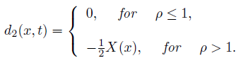
Second, at the points (x, t) where ρ > 1, we have  ≥ 1 − ϵ2 > 0 for a small ϵ2 > 0, and X(x) ln ρ = X(x)(
  (v + s) + M). Then,
 (28)
(28)
Therefore, the first inequality in (22) is proved. Similarly, we may prove the second inequality in (22). Lemma 2.1 is proved.
Since b2(x, t) ≤ 0, d2(x, t) ≤ 0, under the conditions given in (8), it is clear that v(x, 0) ≤ 0, s(x, 0) ≤ 0, so, we may apply the maximum principle (cf. Lemma 2.4 given in [8]) to (22) to obtain the estimates v(x, t) ≤ 0, s(x, t) ≤ 0, and so the estimates in (10).
From the estimates in (10), we can use the Riemann invariants (9) to obtain the following uniformly bounded estimates on (ρϵ,δ(x, t), mϵ,δ(x, t)) directly:
 (29)
(29)
for a suitable positive constant M1, which is independent of ϵ, δ and the time t. The existence result of the Cauchy problem (6)-(7) follows by applying the standard theory on the parabolic systems. Part I of Theorem 1.1 is proved. Furthermore, we may select a subsequence of (ρϵ,δ(x, t), mϵ,δ,µ(x, t)), which converges pointwisely to a pair of bounded functions (ρ(x, t), m(x, t)) as δ, ϵ tend to zero by using the compactness framework given in [3], and prove that the limit (ρ(x, t), m(x, t)) is an entropy solution of the Cauchy problem (1)-(2), so Theorem 1.1 is proved.

