


 Spanish (pdf)
 Article in xml format
 Article references
 Send this article by e-mail
 Cited by SciELO
  Cited by Google
  Similars in
SciELO
Similars in
SciELO  Similars in Google
 Permalink
Introduction
Nowadays a change in the mobility paradigm is emerging regarding the replacement of private usage of fossil-fueled vehicles by more eco-friendly and energy-efficient mobility services, such as the electro-mobility for public transport and the electric car-sharing (Firnkorn and Muller, 2015; Seign, Schussler, and Bogenberger, 2015). Moreover, the adoption of electric vehicles presents an opportunity to provide energy storage-based ancillary services to the power grid, such as supporting grid frequency stability, contributing to the voltage regulation system, and smoothing intermittency due to renewable energy sources (Kang, Duncan, and Mavris, 2013), which is called vehicle-to-grid operation mode (V2G). However, this operation mode imposes additional challenges, such as the management of bi-directional power flows, and the design and implementation of more complex operation strategies that must achieve the economic sustainability of the service. Therefore, it is necessary to propose decision-making tools that allow the operator to take the best economic and operational decisions for the EVs, such as those presented by previous authors (Alkhafaji, Luk, and Economou, 2017; Rabiee, Sadeghi, Aghaeic, and Heidari, 2016; Wu, Yang, Bao, and Yan, 2013). However, these previous works do not consider the batteries wear due to the adoption of the V2G strategy. The wear of the EVs batteries is a critical aspect, as highlighted by Semanjski and Gautama (2016), to reach the satisfactory commercial feasibility of a transport system that involves electric vehicles. As a result, some studies have focused on the inclusion of batteries wear cost when the EVs are featuring the V2G operation mode. Various authors have addressed this issue (Choi and Kim, 2016; Correa-Florez, Gerossier, Michiorri, and Kariniotakis, 2018; Han, Han, and Aki, 2014; Xu, Shi, Kirschen, and Zhang, 2018) using the Achievable Cycle Count function defined by the battery manufacturer, as in Choi and Kim (2016) and Han et al. (2014), or with the Rain-flow algorithm to cycle counting, as in Xu et al. (2018). Authors as Bocca, Chen, Macii, Macii, and Poncino (2018) proposed to use the Arrhenius equation to evaluate the wear of EVs for residential usage and established an optimal charging plan to reduce the charging and wear costs. Nevertheless, all the previous cited studies only calculate the wear of all the EVs aggregated in a set and not individually. The study of Choi and Kim (2016) only considers one EV. These calculations are an approximation, as for a fleet of EVs, each vehicle will have a different wear cost, depending on the routes assignment.
This paper proposes a control strategy for the optimal management of a fleet of EVs that are used to provide public transport services and operate in V2G mode. The proposed control strategy, based on optimization, makes a trade-off between the charging costs of the EVs and the revenues obtained by delivering power to the electric network, considering the battery wear cost of each vehicle in the fleet. The decision variables calculated are the charging and discharging power and the route assignment for each EV. The control strategy is applied to the study case proposed by Ruiz, Arroyo, Acosta, Portilla, and Espinosa (2018).
The contributions of this paper cover two issues. The first one is the individual calculation of batteries wear, i.e. for each EV, which is performed simultaneously with the assignment ofroutes to the EVs in the fleet, and the estimation of charging/discharging profiles. The second issue is the proposal of an explicit mathematical function for calculating the peaks in the energy ofthe battery, which allows counting the charging/discharging cycles using the Rain-flow algorithm.
This paper is divided as follows. The Methodology section describes the theoretical framework and the optimization approach. The section Study case contains the data of the study cases used to compare the wear results and to apply our proposed control strategy. At last, Results and analysis contain the obtained results and their interpretation.
Methodology
In this study, we considered that all the electric vehicles are parked at the same place and that they are connected to the same charging station. Additionally, round-trip travels are assumed. Hence, an EV can be charged or discharged at any moment after finishing the travel.
Figure 1 depicts the structure of the proposed control algorithm. The algorithm is composed of astage of estimation of the required travels and the calculation of the power consumption in them. These procedures are performed by software of traffic microsimulation, entering specific fluxes of passengers at some places (stations of the EVs) in the traffic network. Once the number of passengers that need to be transported to a defined destination point is established, the required departures of the vehicle are calculated. With the calculated route and with a "typical" speed profile, the power consumption of the vehicle is estimated. After the estimation of both variables for a typical day, the estimated data are entered as the input of the control algorithm block.

In the control algorithm block, an optimization is constructed. The aim of this optimization is the reduction of the energy and battery wear costs. The energy cost takes into account the expenses for purchasing energy to charge the EVs and the revenues generated by the delivering power from EVs to the electric network. Furthermore, the constraints include the operational limits of the EVs and guarantee the coverage of the required routes assigning each travel to one of the vehicles in the fleet. The outputs of the optimization are a binary matrix that indicates the vehicle selected to perform each travel and the magnitudes of the charging and discharging powers for each EV and each time step. The mathematical approach used by the constructor of the optimization is described below.
Mathematical approach of the optimization
Objective function and constraints:
First, the decision variables are defined. They are the real-valued matrices P c e ℝnxv that represent the charging power for each EV in the set V = {1,...,v}, where v is the total amount of vehicles in the fleet considering each time step in the set N = {1,..., n} and n is the number of steps in the calculation period; and P d e ℝnxsv that represents the discharging power for each EV. Additionally, the optimization has other two decision variables with binary values. The first one is the matrix A v e ℝrxv whose elements (i, j) have unitary values if the j-th vehicle performs the i-th travel, which belongs to the set of travels R = {1,..., r}. Hence, if vehicle number 4 performs the first travel, then A v (1,4) = 1. The second one is the matrix A c e ℝnxv that indicates if a vehicle is charging and contains unitary values in the positions corresponding to the time steps at which a vehicle is charging.
The objective function is the minimization of the EVs operative costs, which include the expenses for purchasing energy to charge the EVs and the batteries wear cost. Additionally, the revenues generated by delivering power from EVs to the electric network are included. This objective function is indicated in Equation (1).

where p c(i) and p d (i) are the column vectors of the matrices P c and Pd, respectively; w is the wear cost function, Ep e Rn is the electricity price at each time step, and S(¿) are the column vectors of the state of charge matrix S e ℝ (n+1) xv, which is also called SOC and is calculated using the Equation (2) for the i-th vehicle at the j-th time step.

P r e ℝnxv is the matrix that contains the power consumption for the travels performed by each EV at each time step, after each travel is assigned one of the EVs. σ is the self-discharging factor of the batteries and Em, the maximum energy that can be stored in them.
The matrix P r depends on the travels assignment. Equation (3) indicates how to calculate this variable.

C t ∈ ℝnxr is the matrix that contains the power consumption in each travel, which is the output of the urban traffic microsimulation,
Furthermore, the optimization constraints, are shown in Equations (4)-(12):
Pr, P c , and P d must be positive real-valued matrices:

The state of charge of the batteries must be kept between the minimum allowed energy content Sm, and 1.

The total power consumption in the travels at each time step, must be equal to the total power that the EVs spend during their assigned travels each time step:

Travels must be assigned only to one vehicle:

The charging power of the EVs must be kept between 0 and its rated value defined by the manufacturer Pc,m, at the time steps when EVs are charged (indicated by ones in the A c matrix).

The discharging power of the EVs must be kept between 0 and its rated value defined by the manufacturer Pcm, at time steps when EVs are discharged, i.e. when they are not performing a travel or charging

where U ∈ ℝ nxv is a binary matrix calculated with Equation (10). The rows of U correspond to the time steps and its columns to the ID number for each EV in the fleet. This matrix has ones in the time steps when a vehicle is performing a travel, and 0 otherwise.

Being At e ℝnxr a binary matrix that contains ones at time steps where travel is required, it has as many columns as required travels. This matrix is obtained from the output data of the urban traffic microsimulator and entered as the input of the optimization. Furthermore, the sum of the elements of the binary matrix that indicate the charging status and those that show the running status for a vehicle performing travel must be less than 1, as indicated in Equation (11)

Finally, the power charged or discharged from the EVs in the fleet must be lower than the power capacity of the feeder (P;) to which the charging station is connected:

Batteries wear modeling:
The function w in Equation (1) is calculated in two ways:
a) The wear is calculated with the methodology presented by Xu et al (2018) using the Rain-flow algorithm.
This algorithm identifies the peak points of the charging/discharging profile. Then, from, these peak data, the half and complete equivalent cycles from the profile are calculated, using the algorithm detailed by Blumenthal (1935), and entered as inputs of the wear function that is described in Equation (13)

where the constant C¡, takes into account the equivalent present value of the replacement costs for a defined Capital Recovery Factor, and the constants k1, k 2 are defined by the battery manufacturer. The variable A takes a value of 1 for complete cycles, and a value of 0,5 for half cycles.
This study proposes a novel approach to calculate the peak data from the charging/discharging profile in order to compute the Rain-flow algorithm and calculate the sub-gradient of this function for solving the optimization problem with nonlinear methods based on the gradient. The peak data from the charging/discharging profile for the i-th EV and the j-th time step can be extracted using Equation (14)

The logic of the Rain-flow (RF) can be implemented using conditional operators, to identify the halfand complete cycles from the peak data. The objective function is not differentiable at some points, the cycle junction points. Therefore, the subgradient function is defined in Equation (15) based on the approach presented by Xu et al. (2018).

where the points j 1 and j 2 are the cycle junction points between the point j.
However, considering a fleet of more than 1 EV, the nonlinear optimization problem described in Equations (1)-(15) becomes a mixed-integer nonlinear problem. Hence, in order to achieve results with a lower complexity and computation time, the wear calculation is reformulated.
b) The wear is calculated with the Achievable Cycle Count (ACC), based on the approaches presented by Choi and Kim (2016) and Han et al. (2014).
The wear can also be calculated using the cycle life curves of the battery, given by the manufacturer. This cycle life is determined by how deeply the battery is used, i.e. by the depth of the discharge (D = 1 - S). Hence, a relationship between D and the life cycle must be established. In the literature, this relationship is commonly modeled by a polynomial function as in the studies of Choi and Kim (2016) and Han et al. (2014), where the cycle life N cycle is determined with the polynomial function of Equation (16).

where constants a and b are estimated from the manufacturer data. The wear cost is calculated as Choi and Kim (2016):

w d (s) is the wear-out density function, which is calculated as Equation (18) shows:

In Equation (18), the constant Cb takes into account the equivalent present value of the replacement costs for a defined Capital Recovery Factor. Hence, the complete expression for the battery wear is given in Equation (19).

A linear approximation for polynomial expressions is proposed on the integral calculated in the Equation (19). Thus, the approximated wear is:

where p 1 is the slope of the linear function approximating the polynomial expression of Equation (19).
Once the wear function of Equation (20) is considered, the optimization problem becomes a mixed-integer convex problem, whose solution is presented in the Results and analysis section.
Study case
Two study cases are considered. The first one, which is more reduced than second, is used to compare the wear obtained using both proposed approaches. The second study case, which contains the data demand described in Ruiz et al. (2018), is used to apply the proposed control algorithm for a fleet of EVs.
First study case:
The first study case considers one electric vehicle, a Renault Twizy. The travels performed by the EV in the evaluation period are predicted from the behavior of co-housing users described by Semanjski and Gautama (2016). The operating hours of this vehicle are between 5:00 and 16:00. The energy consumption in each travel is calculated with the daily travels, which are generated randomly. The random generation of daily travels uses a normal distribution for the distance of each travel and the number of travels per day, taking into account the next parameters: a daily average traveled distance of 8,4 km, and a daily average of travels performed of 3. Three days were simulated. The parameters considered for the wear function were taken from the study of Correa-Florez et al. (2018) and are presented in Table 1.

Hence, with the energy consumption data already calculated, this study case only requires the execution of the steps indicated in the Control Algorithm block in Figure 1. The optimization, including the wear cost, was solved using Matlab 2015b. Three optimization cases were taken into account: the first case without considering the wear cost, the second case using the Rain-flow algorithm to calculate the wear cost, and the third case that includes the wear cost and uses the ACC function to calculate it. The solutions of the first and third optimization problems were found with the CVX optimization tool and the Gurobi solver, as both are convex problems. Gurobi uses the Branch and Cut algorithm. The solution of the second case was found using the fmincon function of the MATLAB Optimization Toolbox with the Active-Set optimization algorithm.
Second study case:
The study case used to apply the algorithm of Figure 1 includes the traffic network, and the passengers demand described by Ruiz et al. (2018), which presents a study case applicable for the city of Medellfn, Colombia. The urban traffic microsimulation to calculate the required travels and power consumption in them was performed using the software SUMO. The electric vehicles considered are BRTs Type 1, as described in Ruiz et al. (2018), whose energy capacity is 324 kWh. The data of the required travels and power consumption in them were taken from Ruiz et al. (2018), taking into account only the travels performed by BRTs Type 1. The electricity price time series and the power limit for the feeder of the charging station were also taken from the aforementioned study.
The parameters considered for the evaluation of the batteries aging are presented in Table 1 with a replacement cost of batteries of USD 5 400. This wear calculation was done only with the ACC approach, using Equation (20). Time steps of 10 minutes were considered, a simulation period of 24 hours, a fleet size of 5 BRTs, and 21 travels required to cover the passenger demand. The software used to compute the optimization was Matlab 2015b with the Gurobi solver.
Results and analysis
Results for the first study case:
Figure 2 illustrates the SOC of the battery without considering the wear, considering the wear and calculating it with the Rain-flow algorithm (RF) and with the Achievable Cycle Count ACC.

Source: Authors
Figure 2 Comparison of the SOC for the different presented approaches for the wear calculation.
The value of the wear is USD 0,04 calculated with the integral of the ACC, and USD 0,07 with the Rain-flow algorithm.
Figure 2 shows the SOC for the wear calculated with the Rain-flow algorithm. The result is more conservative compared with the other cases, because the Rain-flow algorithm performs two approximations. The first approximation evaluates the wear function for the difference of SOC between two points, instead of calculating the difference of the wear function evaluated at two different points, as in the wear density function presented in Equation (19). The second approximation is the cycle account, in which the non-peak data from the SOC profile is neglected, and half cycles are added. In addition, to extend the Rain-flow algorithm for a fleet of EVs, the use of Mixed-Integer Nonlinear optimization methods is required, which have a higher computational complexity than methods based on Mixed-Integer Linear Programming.
The computing time was 379 seconds for the wear calculated with the Rain-flow algorithm, and 6 seconds using the linear approximation for the integral of the wear density function. Hence, for the second study case, the wear density function is used.
Results for the second study case:
The SOC for the fleet of EVs is illustrated in Figure 3. This Figure shows that the SOC of all the EVs in the fleet increases around the time intervals 2:00 - 5:00, and 16:00 - 18:00. Those intervals correspond to the lowest electricity price hours for non-operating hours, i.e. the vehicles are charged at hours when the electricity is cheaper.

Furthermore, from the results shown, it can be concluded that allowing the V2G mode, the fleet operating costs are reduced by 50%. The obtained average SOC for the EVs in the fleet is illustrated in Figure 4, without considering the batteries wear cost and considering it.
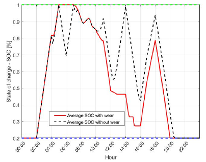
Source: Authors
Figure 4 Comparison of the average batteries SOC with and without the inclusion of the wear cost.
The average SOC presents a peak reduction considering the wear cost. This smoothing in the SOC impacts on the revenues that can be obtained by delivering power to the electric network, since the charging/discharging power cycles are more constrained and generate an overrun cost of USD 0,59 per day. This overrun cost is compensated with the savings in the batteries wear, which represents 26,03 % of the operating costs. The obtained error compared with the non-approximated wear cost presented in Equation (19) was 20,7%, which is equivalent to USD 0,01 per day.
Conclusions
This paper presents a control strategy to manage the charging and discharging power of a fleet of EVs that participate actively with the power network in V2G mode. This control strategy includes the wear of batteries in the operative costs, which are minimized. Two approaches were used for the wear calculation: the Rain-flow algorithm and the integral of the wear density function. Also, the control strategy, considering the integral of the wear density function, was applied to a fleet of EVs for the individual calculation of batteries wear, which is performed simultaneously with the assignment of routes to the EVs in the fleet and the calculation of charging/discharging profiles. Results showed that with the inclusion of the wear cost, the V2G mode is still profitable, but the revenues of the fleet operator are reduced to half approximately. The Rain-flow method delivers more conservative results for the wear estimation since it counts half cycles, but the ACC method allows the linearization of the optimization problem.
Hence, a lower computational complexity is required to solve the optimization problem.
Additionally, the proposed control strategy depends on the parameters of the wear function given for the battery. This function must be approximated applying operative tests. Hence, to extend the proposed strategy the validity of the wear parameters must be verified for the batteries of the considered fleet.


