


 English (pdf)
 Article in xml format
 Article references
 Send this article by e-mail
 Cited by SciELO
  Cited by Google
  Similars in
SciELO
Similars in
SciELO  Similars in Google
 Permalink
Introduction
Landslides are strongly related to rainfall events as a triggering factor (Chien, Hsu, and Yin, 2015), which mainly cause shallow landslides. Landslide hazard is evaluated as an instrument for territorial planning, decision making, contribution to the state of the art, and a component of risk assessment. It has also been studied under the guidelines of heuristic, probabilistic, statistical and empirical methodological approaches (van Westen, van Asch, and Soeters, 2006). However, a deterministic landslide modeling approach can be more reliable to assess and analyze the physical processes that govern the issue of slope instability, generally associated with changes in the stress state of the soil.
These changes are due, among other factors, to the hydrogeological conditions of the soil, expressed in terms of variations in the position of the water table or changes in pore pressures caused by the intensity of rain precipitation. Thus, events of less intensity (longer duration) are associated with changes in the position of the water table, which causes deep landslides; and events of greater intensity (shorter duration) are associated with changes in pore pressures, which causes shallow landslides (Ran, Hong, Li, and Gao, 2018; Aristizábal, Martínez, and Vélez, 2010).
Shallow landslides should be assessed considering that the infiltration of the rain is the main triggering factor that generates slope instability, and its study should lead to determine variations in the groundwater regime that generate changes in the safety factor (Iverson, 2000). The Iverson model allows evaluating the redistribution of underground pore pressures associated to the transitory infiltration of the rain and its effects on the time and location of landslides. In addition, the use of geographic information systems (GIS) allows the spatial and temporal distribution of safety factors and their classification to generate hazard maps.
This paper aims to show the guidelines for the generation of hazard maps according to shallow landslides associated with infiltration processes by means of a deterministic approach, using the Iverson model (2000) at a regional scale in the Sapuyes river basin. The data of the study area were obtained from studies carried out by entities such as IGAC, IDEAM, SGC, Corponariño, and they were processed with a GIS. The Iverson model was used to calculate pressure heads and safety factors into cells of 12,5 m, according to the resolution of the Digital Elevation Model (DEM) through an open access software (GRAS GIS). Finally, the safety factor was classified into ranges that allowed visualizing the hazard level.
Materials and methods
Study area
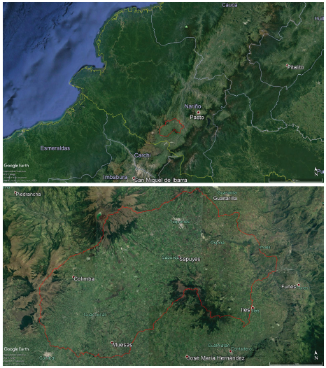
The study area was the Sapuyes River basin in the department of Nariño, located approximately between the geographical coordinates 77°48'20"W - 00°54'16"N and 77°28'30"W-01 °07'55"N. It has an approximate area of 515 km and an average elevation of 3314 meters above sea level. There are 8 municipalities in the region, as well as the main route between Tumaco port and Pasto city. Figure 1 shows the location of the study area at regional and local revels.
Resources
The resources used in the deterministic evaluation to create hazard maps are presented in Table 1.
Methodology
Background: Scientific literature and research papers were reviewed to identify a physical model which considers variations in the pressure head as a factor that generates instability, with an analytical solution and minimum input parameters.
Model identification: The Iverson model was chosen to perform the hazard modeling. Iverson (2000) uses rational approximations to develop a theoretical model by means of the effective stress principle in an infinite slope stability analysis, while also considering the redistribution of subsurface pore pressures associated with transient rainfall infiltration, in order to evaluate the effects of rain on time and location of landslides.
The analytical solution of the Iverson model to calculate pressure heads (Ψ) is shown in Equation 1, whereas Equation 2 is used to calculate safety factors (FS).
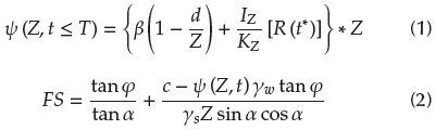
where d is the water table depth measured normal to the ground surface, Z is the soil depth, I z is the rainfall intensity, Kz is the soil hydraulic conductivity, φ is the soil friction angle, α is the slope angle, c is soil cohesion, γ w is the unit weight of groundwater, and γ s is the soil unit weight.
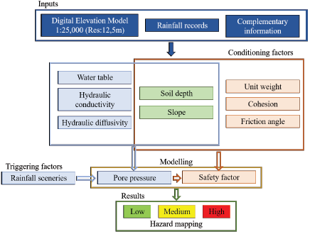
Treatment of input data: The parameters of the Iverson model were grouped into conditioning and triggering factors. Among the conditioning factors are the properties of the slope and the soil, while the triggering factor is rainfall intensity.
The DEM obtained from satellite images was processed to obtain and make correlations between the hillside slope and the stratum soil thickness . From IGAC information, the physical properties of the soil such as hydraulic conductivity and diffusivity, and unit weight were correlated, as well as mechanical properties such as cohesion and internal friction angle.
The rainfall data were processed to obtain equations of intensity i = C0 * TC1 r * D C2 from meteorological stations in the study area. All the obtained information was spatially distributed using a GIS. Some parameters (φ,c,K Z ,γ s ) were assigned to the soil units of the IGAC, and others were interpolated (Z,I Z ,d).
Modeling: The Iverson model was programmed in GRASS GIS to calculate pressure heads, safety factors, as well as to classify the hazard.
Hazard mapping was carried out by classifying the safety factor based on the values in Table 2.
Table 2 Hazard categories
| Level | Safety factor |
|---|---|
| Low hazard | > 1,5 |
| Medium hazard | 1,1 -1,5 |
| High hazard | < 1,1 |
Source: Modified from /Avila et al. (2015).
Also, an additional classification of the maps was made to show unstable slopes with a factor of safety of less than 1,0.
The flow diagram in Figure 2 explains the guidelines for hazard mapping in general terms.
Results
The hillside slopes map (Figure 3) showed an average slope of 12°; 51% of the slopes have values between 0° and 10°, 31% between 10° and 20°, 12% between 20° and 30°, and 6% greater than 30°.

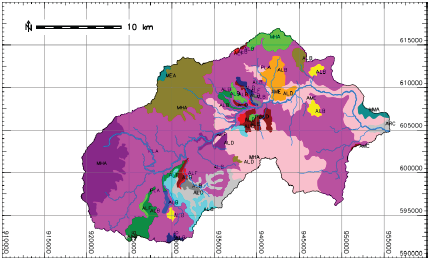
Ten soil units were identified (Figure 4), and physical and mechanical properties were assigned based on the soil study of the department of Nariño (IGAC, 2004).
For each meteorological station (Figure 5), a time series was generated, an approximated extreme values (Gumbel) probability distribution function was made, and a multiple linear correlation was performed to obtain the intensity parameters (Co, C 1 , C 2 ).
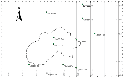
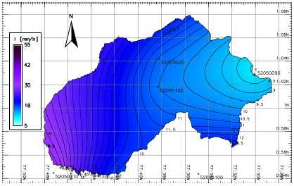
Figure 6 shows a rain intensity map and isohyets generated for a 30-minute rainfall and a return period of 2,33 years. Likewise, intensity maps for return periods of 2,33, 20, and 100 years were generated, a s well as rainfall durations of 30, 60, and 120 minutes.
Pressure head
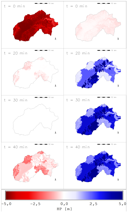
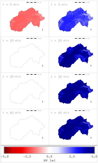
Pressure head changes, as a function of the depth and evaluation time in an individual cell (Figure 7), show the quick response of the pressure head in a depth equal to the soil stratum depth. This can be observed in the spatial distribution map (Figure 8). The pressure head evaluated at the depth of the soil layer does not strictly represent the most critical condition, that is, the highest pressure head.
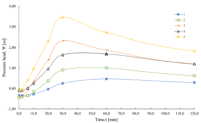
Both the spatial distribution of the pressure head (Figure 8) and the pressure head in individual cells (Figure 9) with different parameters, show the maximum condition of the pressure head around at t = 30 min, when the rain has already ended. In addition, although thinner soils develop smaller pressure heads than thicker soils, hydraulic diffusivity can generate changes in the pressure head for soils of equal thickness.
Source: Author
Figure 8 Maps of the spatial and temporal distribution of the pressure head: Left) on the surface, Right) at the depth of the soil layer.
Source: Author
Figure 9 Temporal changes of head of pressure on individual slopes for a rain of 30 minutes in 5 individual slopes.
Figure 10a shows the maximum sustainable pressure head with a water table located at a depth of 2,0 m, which, at a time t > 0 min, cannot exceed the hydrostatic pressure in any case. Aditionally, Figure 10b shows heads of pressure greater than those observed when the water table is located at a 5,0 m depth (Figure 8). It indicates that the position of the shallow water table generates a pressure head greater than at a deeper water level.
Source: Author
Figure 10 Maps of the spatial and temporal distribution of pressure head with water table located at 2 m depth: Left) on the surface, Right) at the depth of the soil layer.
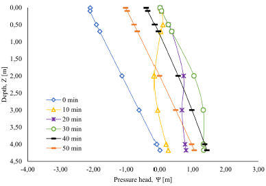
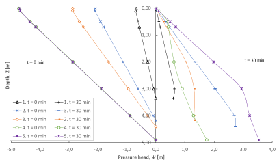
Pressure head variations at different evaluation depths were evinced when the water level was located at the same depth of the soil stratum. It could also be observed that the pressure head is equal to the hydrostatic pressure at the surface of the soil layer at the end of the rain (t = 30 min) and at the depth of the soil layer at the beginning of the rain (t = 0 min). Negative pressure heads at t = 0 min indicate suction in the soil, while positive pressure heads are developed at t > 0 min. This tendency is more evident when the pressure head is evaluated on individual slopes (Figure 11). It is also seen that, in some slopes, the response of the pressure head is associated to the hydraulic diffusivity of the soil. In other words, soils with lower hydraulic diffusivity may have lower pressure heads (Figure 11, point 4).
Source: Author
Figure 11 Response of the pressure head on individual slopes at the beginning (left) and at the end (right) of the rain.
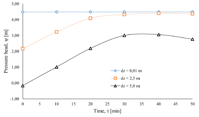
Figure 12 shows the changes in the average value of the pressure head at the same depth of the soil stratum for different positions of the water table. In general, the pressure head is greater when the position of the water table is superficial, and lower when the position of the water table is located at a greater depth. In addition, the response of the pressure head is greater when the water table is deeper.
Source: Author
Figure 12 Changes of the pressure head as a function of the depth of the water table.
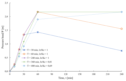
Once the rain has finished, the response of the pressure head decreases in an approximately parallel way (Figure 13). In addition, in soils with low hydraulic conductivity, the ratio Iz /K z > 1,0 generates an equal pressure head for different rain durations (different intensity), since Equation 1 is only conditioned in this case by the response function R(t*). In the same way, it was identified that, in soils of low hydraulic conductivity, increases in rainfall intensity with the return period do not generate changes in the pressure head.
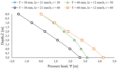
When the ratio
 = 1,0 (low permeable soils and high rainfall intensity), the response of the pressure head is equal for rains of any duration until the moment the rain ends. Furthermore, when the ratio Iz
/K
z
< 1,0, the response of the pressure head is different during and after the rain (Figure 14).
= 1,0 (low permeable soils and high rainfall intensity), the response of the pressure head is equal for rains of any duration until the moment the rain ends. Furthermore, when the ratio Iz
/K
z
< 1,0, the response of the pressure head is different during and after the rain (Figure 14).
Source: Author
Figure 14 Response of the pressure head of an individual slope for rains of different duration.
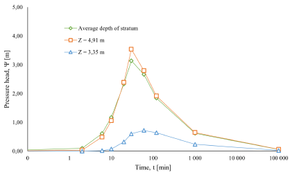
In addition, the time for the pressure head to return to its initial condition tends to be greater for longer duration rains, i.e. it depends on the duration of the rain (i.e. for a 30-minute rainfall the estimated time for the pressure head to return to its initial condition is 100 000 minutes (70 days) at any depth of evaluation) (Figure 15).
Factor of safety
Figure 16 shows that FS changes for different rain evaluation times, and smaller FS values can be identified when t ~ T (30 min). Increases in FS evaluated at t > T are presented by the reduction of Ψ at t > T (Figures 8 and 10).
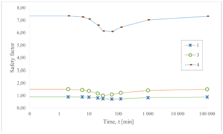
Although the safety factor can be recovered and returned to its initial condition over time (Figure 17, line 4) like the recovery of the pressure head, the same analogy should not be made once the slope has reached failure (Figure 17, lines 1 and 3), and the analysis is performed until the time when FS ≤1,0. Therefore, a suitable way to interpret the variations of FS as a function of t is to analyze until the moment in which the minimum value of FS is reached, considering that this moment is close to the duration of the rain.
Due to the fact that minimum FS values do not occur at the same time on all slopes, since some may fail at different times, Figure 18 shows the minimum FS value for each slope, found from the evaluation of FS at different times. Figure 19 shows the FS decrease until an instant t ~ T. Additionally, it can be observed that the safety factor is recovered after the rain has finished. In this sense, the FS value corresponds to the minimum FS values evaluated at t = 0,10,30,40,60 min.
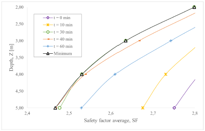
Source: Author
Figure 19 Changes in the safety factor according to the depth and time of evaluation.
In Figure 20, variations in the average FS values associated with the initial position of the water table (d z ) can be observed. Lower values of FS occur when dz is more superficial, and there are greater values when dz is deeper. On the other hand, a trend of minimum FS values is observed in moments close to T. In addition, the FS variations over time remain almost constant for surface values of dz and decrease more quickly for deeper values of dz.
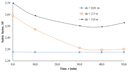
Source: Author
Figure 20 Changes in the factor of safety with variations in the position of the water table.
Thus, it can be inferred that the response in slope stability is directly associated with the location of the water table in the slope. Therefore, in slopes with a shallow water table position, the safety factor remains almost constant during and after the rainfall duration. An FS value that does not change over time means that the slope always remains in its original condition (stability or instability).
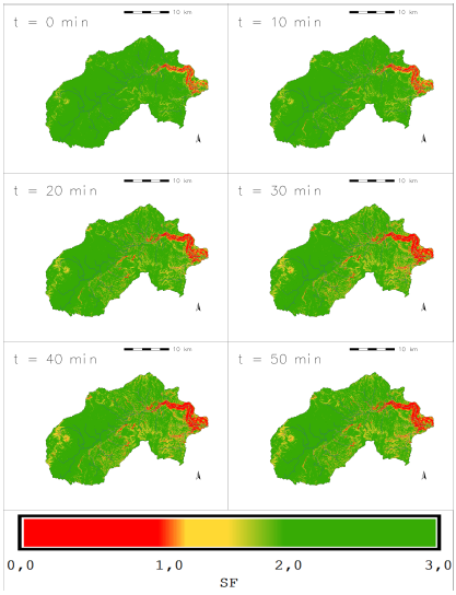
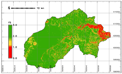
Hazard mapping
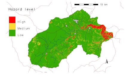
The mapping of hazard as a time function is presented for the instant in which the safety factor is at its lowest in each slope (cell) at all evaluation times (Figure 18). Figure 21 shows the hazard map by FS classification according to the criteria of Table 2; the scenario considers the minimum FS value for all the evaluation times.
Discussion
The spatial distribution maps of Ψ(Z, t) show the response of the pressure head for high intensity rain events (Iz) and low hydraulic conductivity soils (Kz), i.e. I z /K z ≥ 1. Furthermore, the maximum pressure head develops very closely to the duration of the rain at times (Figure 14). The above is observed in a similar way by the determination of pressure heads for maximum precipitation events from instrumentation with piezometers (Fannin et al., 2000). The temporary variations of the pressure head, under different ratios Iz/Kz determine the stability of the slope, because soils with greater hydraulic conductivity generate more positive pore pressures. In this way, the factor of safety at different depths decreases the lower the value of Iz/Kz (Zhang, Zhu, and Zhang, 2020)
Although the pressure head evaluated at the end of rain is less for a higher intensity rain (Figure 13) in soils with an ratio Iz/ Kz = 1 , when the ratio Iz/ Kz ≤ 1 is obtained higher pressure heads for higher intensity rains (Figure 14) (Zhang et al., 2020). In fact, measurements of pressure heads from instrumentation with piezometers also show this behavior (Fannin, Jaakkola, Wilkinson, and Hetherington, 2000). This is related to the generation of positive pore pressures and the occurrence of surface landslides associated with periods of high intensity rainfall (Sidle and Ochiai, 2006; Aristizábal, Martínez, and Vélez, 2010; Cho, 2009). Likewise, the pressure head variation rate in terms of depth is at times equal to or greater than at the end of rain (Figure 14), that is, pore pressure tends to dissipate steadily throughout the range of depth. According to Ivanov et al. (2020), there is an inverse correlation between Iz/Kz and the slope's time of failure, implying that higher intensity rainfalls need less time to cause failure. This is directly related to the development of higher pressure heads, which will cause decrease soil strength and the fall of slopes as well.
The analysis of short-term duration rainfalls with the Iverson model implies that the hydraulic diffusivity value applies for conditions close to soil saturation, while the recovery of the pressure head with time implies a decrease in soil saturation for instants after the end of the rain. Thus, it can be concluded that the recovery time of the pressure head is more associated to hydraulic diffusivity than to the duration of the rain (Figure 14).
Both Figure 15 and Figure 17 indicate that the pressure head and the safety factor tend to return to their initial condition after very long periods of time (70 days). However, the prediction made may not be significant, considering that the Iverson equations are considered for short evaluation periods, as well as the fact that it differs from observations made with piezometers (Fannin et al., 2000), in which it is observed that pressure heads return to their initial condition after much shorter times.
The spatial distribution of the safety factor (Figure 16) is closely related with pore pressure variations. In addition, these variations in the FS are observed both in the analysis of an individual slope and in the spatial distribution. In fact, the spatial distribution of the safety factor and its relationship with pore pressures can be studied through the application of deterministic models that perform a physical analysis of the problem (Kim, Im, Lee, Hong, and Cha, 2010; Baum, Godt, and Savage, 2010).
Pradel and Raad (1993) stated that surface failures are more likely to occur in sandy or gravel soils (high hydraulic conductivity), but there is a higher potential for failure in silt and clays (low hydraulic conductivity) in natural slopes, i.e. the influence of hydraulic conductivity on slope stability is not clear. Similarly, downscale tests in sands have showed that hydraulic conductivity (Kz) is a parameter that governs soil stability, considering that soils with a higher void ratio allow a quicker redistribution of rainfall water (Ivanov et al., 2020). However, taking into account that FS variations depend on variations in Ψ(z, t) and, in turn, variations in Ψ (z, t) depend on the hydraulic conductivity of the soil (Ksat) and rainfall intensity (Iz), it is possible that large variations in Ψ (z, t) are not observed for higher rainfall intensities, since the water response is conditioned by the Iz/Kz ratio.
Some authors refer to shallow landslides as those in which the sliding mass has a thickness between 2,0 and 3,0 meters (Baum, Godt, and Savage, 2010; Anderson and Sitar, 1995), while others refer to a depth less than 2,0 meters to consider a surface-type slip (Pradel and Raad 1993; Iida, 1999; Schiliro, Montrasio, and Scarascia Mugnozza, 2016; Aristizábal et al., 2010; Chae, Lee, Park, and Choi, 2015). Although it is not easy to define a single criterion for the classification of shallow landslides, the simulations of the safety factor allowed observing that most of the slopes failed for an evaluation depth of less than 3,0 meters under the considerations of this case study.
Regarding the results, physics-based deterministic methods that explain the variations in the groundwater regime (Kim et al., 2010; Montrasio and Valentino, 2008) are similar to those obtained through the methodological application made in this investigation for obtaining hazard maps. The current approach allows to consider the dynamics of the hydrologic events from real rainfall intensity values (Iz) and temporal variations, which play an important role for the development of instability (Ivanov et al., 2020)
Some deterministic approaches and methodologies for the evaluation of landslide hazards (Avila et al., 2015; Westen and Terlien, 1996) calculate the FS by assigning a water table height that is related to the amount of rainfall that precipitates for different periods of rain or return periods. Although these approaches have valid physical assumptions, they are not the most adequate for the evaluation of the physical process that conditions the instability of the slope. Additionally, the application of the models in question does not allow evaluating the temporal variations of the safety factor.
Furthermore, the proposed approach allows evaluating infinite scenarios based on the variables of the Iverson model (2000), mainly as a function of rainy weather, that is, during the entire duration of the storm, or even after it.
Conclusions
The possibility of performing temporary analyses of variations in the pressure head and the safety factor in slopes was identified as one of the main advantages of the methodological approach used in this study. Compared to other methodologies, temporality is a relevant factor when you want to deepen the knowledge of the process that leads to slope instability in periods of time that are approximately equal to the duration of the precipitation event.
It was determined that pore pressure modeling is very sensitive to variations in the initial location of the water table. Therefore, in the subsoil exploration stage, an additional effort must be made to determine the depths of the water table and make an adequate spatial distribution of the data.
Based on the results of the safety factor for different soil thicknesses, it was determined that a good criterion for the classification of surface landslides (~ 3,0 m) results from the application of deterministic models for FS spatial distribution.
The hazard assessment of landslides associated with changes in pore pressures indicates potentially unstable areas in the Sapuyes River basin. Hazard mapping did not include the validation of the Iverson model, which could be carried out based on landslide inventories, with databases such as the Mass Movements Information System (SIMMA). The validation of the model implies a sensitivity analysis to determine the rate of true positives (Nguyen, Lee, and Kim, 2019).

