1. Introduction
The local failures generated by earthquakes, in turn induce vibrations of the soil. These waves cause the vibration of buildings located in the environment of the epicenter of the earthquake [1]. Several methods have been proposed to evaluate the seismic structural performance in the development of performance-based seismic engineering. The fundamental question is to determine the seismic demand and the capacity of collapse proportional to the Grounds accelaration caused by earthquakes.
Different approaches for assessing structural collapse capacity with the aim to preserve life safety differ from the simplest approach, based on a simple single-degree-of-freedom (SDOF) response model to complex nonlinear dynamic analyses done in a structural model, which is analysed for ground motion records [2].
The capacity spectrum method is highly used. The seismic action is defined by means of the elastic response spectra, the fragility of the building by means of the capacity curve. The latter is calculated from an incremental nonlinear static analysis, commonly known as "Pushover Analysis" [3-7].
With the growth in computational power, new complex analysis tools have been developed to calculate nonlinear response of structures to ground motions. The procedure is accessible for preparation of analysis models, which can capture nonlinear behavior of most components.
Nonlinear time history analysis (NLTHA) tools are becoming regularly available to engineers. This method evaluates structural seismic performance by applying a series of ground motion acceleration induced to the structure. The inelastic earthquake response of a concentrated plasticity model of a building can be greatly affected by how damping is defined [8]. The modeling of damping is a difficult task in dynamic nonlinear analysis [9] caused by the diversity of mechanisms that may be present at once in the damping of the structure [10]. In the inelastic time history analyses of structures in seismic motion, part of the seismic energy that is imparted to the structure is absorbed by the inelastic structural model, and Rayleigh damping is commonly used in practice as an additional energy dissipation source [11].
Energy dissipation and ductility are part of diverse parameters that influence viscous damping ratio [12,13]. The viscous damping matrix is fundamental in nonlinear time history analysis to calculate the inelastic deformation. The effect of viscous damping on the response of the structure is greater than the hysteresis damping connected to the inelastic deformation in the case of moderate earthquakes. Therefore, a correct evaluation of viscous damping and its effects in structural dynamics and earthquake engineering is essential [14].
Early research on damping modeling problems in inelastic structures dates back to the work of [15-17].
The variation of the non-linear response indicators through the average ductility, hysteretic-to-input energy ratio and the average number of yield incursions, as a function of the additional damping model used in the case of inelastic frame structures in seismic loading have been studied by [18].
A capped viscous damping formulation to overcome some of the problems pointed out was proposed by [19] where the use of Rayleigh damping can lead to damping forces that are unrealistically large compared with the restoring force on practical situations.
Charney [17] investigated the effects of global stiffness changes on the seismic response of a five-story structure when Rayleigh damping is used. [17] also investigated the effects of local stiffness changes at the seismic structural time-history response when initial stiffness-based Rayleigh damping is used [11]. Each structural element with an equivalent combination of an elastic element with initial stiffness-proportional damping and yielding springs at the two ends without stiffness-proportional damping was investigated and modeled by [20].
Erduran [21] used tangent stiffness-based Rayleigh damping models to analyze their effect in the story drift ratios, floor accelerations, and damping forces in three-story and nine-story steel moment-resisting frame buildings for three seismic hazard levels [11].
The aims of this article are: (1) to assess the effects of the Rayleigh damping models on the results of nonlinear time history analysis and (2) to demonstrate the impact of the damping model on the assessed engineering demand parameters and conclude by the proposal of a modeling solution appropriate for RC buildings to the RPA 2003 code.
To that aim, the article is organized in five sections; Section 1 introduces the problematic studied in this paper. Section 2 focuses on the presentation of damping in nonlinear time history analysis. Section 3 is devoted to the presentation of the finite element model used in this study. In this section, the viscous damping will also be applied to the case study using different types of approaches to model the damping matrix C.
Section 4 aims to present the main results of the sensitivity analysis. Finally, we end the article with a conclusion based on the observations in the previous section.
2. Damping in time-history analyses
In earthquake engineering, damping is usually present as a ratio or fraction of critical damping, called the damping ratio ξ, which is a property of the system material and independent of its mass and stiffness [12]. The equivalent viscous damping is the sum of the elastic and the hysteric damping [22]. Damping values depend on the construction materials, vibration amplitude, fundamental period and mode shapes, type of connections and the building configuration [23].
Many studies [24-32] have been interesting to draw the exact definition and estimation of equivalent viscous damping.
Experimental investigations have shown that the vibrations of real structures usually lie between the viscous and frictional responses. However, the viscous assumption is convenient to use analytically and is sufficiently accurate for most purposes [33]. The damping of the structure is assumed to be viscous and frequency dependant for the sake of convenience in the analysis. The most popular method is to solve the equation of motion using the modal analysis; in this case, damping values are directly assigned to the modes [34]. Damping ratios can be calculated using the Caughey series [35] which Rayleigh damping [36] is a special case.
Rayleigh damping can be used in seismic simulations either to account for energy dissipation mechanisms that are external to the structure or for energy absorption mechanisms that are internal to the structure [37].
In Rayleigh damping, the damping matrix is a linear combination of mass-proportional and stiffness proportional damping terms as shown in Equation (1):
Where ( and ( are real scalars with 1/sec and sec units respectively. Modes of classical damped systems preserve the simplicity of the real normal modes.
These coefficients have been evaluated from two specified damping ratios ((i and (j) and natural frequencies (ωi and ωj) corresponding to two “references” modes (i and j) of vibration, respectively as shown in Equation (2).
Another important aspect is which characteristics of the structure, initial or inelastic, are used in the computation of the damping matrix. The damping matrix can be constructed by using the initial stiffness matrix Ko, which is constant throughout the analysis, or the tangent stiffness Kt, which is updated at each time-step following the stiffness changes. The values of the constants α and β are based on initial characteristics, which constitutes a computational convenience on the ground that the evolution of the frequency spectrum is not known. The choice of initial damping model between a constant damping matrix and tangent-stiffness proportional damping matrix could be significant, particularly for short-period structures [38]. With initial stiffness elastic damping, the damping coefficient is constant throughout the analysis, even in the inelastic range of response, and is based on the initial elastic stiffness. With tangent-stiffness damping, the damping coefficient is proportional to the instantaneous value of the stiffness and it is updated whenever the stiffness changes [39].
3. Finite element modeling
3.1 Case study
The case study is a 3-story RC frame building designed according to reinforced concrete code BAEL 91 and Algerian seismic code RPA 99/Version 2003 with the following parameters: zone of moderate seismicity, zone Z IIa. A seismic behavior factor of R = 5 was taken into account for reinforced concrete frames without masonry infill.
The Algerian paraseismic code RPA99/version2003 [40] was used for the pre-dimensioning of cross sections of columns and beams. Then, it was used to consider the seismic action as an accidental action in the sense of the limit state calculation philosophy.
Finally, this code was used to determine in beams and columns:
The minimum and maximum percentage of longitudinal reinforcement
The minimum length of recovery
The minimum transverse reinforcement
The BAEL91code was used to calculate longitudinal and transverse reinforcement in beams and columns.
The building has a rectangular plan configuration as shown in Figure 1. The dimensions of the building are 16.6 m long and 8.8 m wide with a total height of 9.18 m in elevation and all the floors are the same height of 3.06 m.
Concrete characteristic compressive strength equal to fck = 25 N/mm2 and steel characteristic yielding strength equal to fyk = 400 N/mm2 are adopted. The member cross-section sizes and steel bars are given in Table 1.
3.2 Numerical Modeling of structural element
To perform time history analysis, frames are modeled in SeismoStruct-V-6 [41] finite element software that is able to perform nonlinear dynamic analysis.
A uniaxial model that follows the constitutive relationship proposed by [42] and the cyclic rules proposed by [43] representing the concrete. The confinement effects provided by the lateral transverse reinforcement are incorporated through the rules proposed by [42] whereby constant confining pressure is assumed throughout the entire stress-strain range. The model adopted for the steel reinforcement is based on the Menegotto-Pinto [44] model coupled with the isotropic hardening rules proposed by [45].
The modeled structure is shown in Figure 2. The beams were divided longitudinally into 4 elements and each beam and column element was divided transversely into 200 by 200 fibers elements.
The capacity curve of the buildings obtained from nonlinear static (pushover) analysis under an invariant first mode load pattern is represented in Figure 3.
3.3 Ground motion selection earthquake
Ground motions observed at a definite site usually depend on the type of the earthquake (fault mechanism, the way seismic wave propagation) [46]
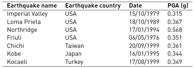
A suite of ground motion records needs to be selected to perform nonlinear time history analysis [Figure 4]. Selected ground motions are shown in Table 2.
Two sets of ground motions that are representative of different intensity measures are used in the response history analysis. The first set represents a moderate seismic zone (zone IIa) and the second a high seismic zone (zone III). The ground motion set selected is scaled to represent ground motions with a RPA99/V.2003 elastics designs spectrum's zone IIa and zone III.
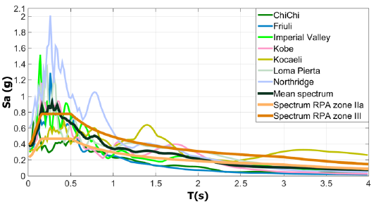
Figure 4 Acceleration response spectrums for the selected earthquakes together with the RPA99/version2003 elastics designs spectrums
The SeismoMatch software [47] was used in the ground motion scaling. It has the ability to scale ground motion acceleration to match to a given target response spectrum. That consists of three steps. First, load all ground motions to the SeismoMatch software as a single ground motion or multiple ground motions. Second, define a target spectrum in the software or load user defined target spectrum of the software. Third, enter interval that needs to match such as 0.2T1 to 1.5T1 and enter a scale factor if available.
Two sets of ground motions satisfy the Eurocode 8 [48] provisions:
The mean of zero period spectral response acceleration values should not be smaller than the value of S.ag (S is the soil factor, ag is the design ground acceleration); in the range of periods between 0.2T1 and 2T1, where T1 is the fundamental period of the structure, in the direction where the accelerogram is applied, no value of the mean 5% damping elastic response spectrum, calculated from all time-histories should be less than 90% of the corresponding value of the 5% damping elastic design spectrum.
3.4 Modeling of viscous damping
The application of viscous damping was only to the building superstructure with the use of many different of computing the damping matrix C that covers a wide range of options available in many existing FE programs [Table 3]. The Table 3 also shows the relevant frequencies obtained from modal analyses.
Approach 1 used the fixed-base frequency of the superstructure to calculate the damping coefficient β. This coefficient remained constant throughout the analysis. Consequently, the damping matrix C remained also constant. In the approach 2, the modification of stiffness allows updating the damping matrix C at each step of the analysis. Approach 3 used the fixed-base frequency of the superstructure in order to compute the damping coefficient α. This coefficient remained constant throughout the analysis. Therefore, the damping matrix C also remained constant.
On approach 4, Rayleigh damping was used where the initial stiffness matrix was used to calculate the damping matrix C by Equation 1.
First and sixth mode frequencies are used to calculate the damping coefficients. This is explained by the fact that the first six modes were observed to contribute to the response significantly after a modal analysis. In approach 5, the same approach is used with a tangent stiffness matrix to calculate the damping matrix.
At last, reduced frequencies as used in Models 6 and 8, in according with the recommendations of [17], who allows us to suppose that the definition of Rayleigh damping based on reduced modal frequencies to account for yielding in these modes. Results are then more reasonable concerning the response evaluation for buildings that are estimated to deform outside their elastic limit.
The 5% Rayleigh damping is used; first and sixth frequency modes are reduced (wi = 0.707w1 and wj = 0.707w6).
Figure 5 shows the damping ratio versus frequency curves for different approaches with the damping coefficients α and β computed using ζ=5%.
4. Discussion and result
The selected Engineering demand parameters include maximum floor displacements, maximum story shear forces and maximum inter-story drift ratios. The ratios of damping forces to mass forces are identified to recognize the damping models that may have as potential results, irrationally high damping forces.
4.1 Damping forces
Figure 6 illustrates the mean values of peak damping force/mass force ratios. This result was obtained by the use of different damping approaches for two seismic intensity measures.
The Ratio of damping force to mass force was observed to identify the damping models which may have as potential results, unreasonably high damping forces [21].
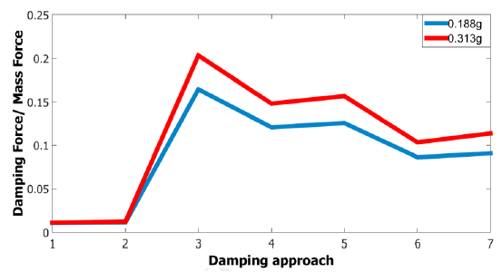
Figure 6 Damping force to base shear force ratio for several damping models for two seismic intensity measures
Figure 6 shows that the damping force/mass force ratio growth with an increase in the seismic intensity for all the damping models considered for the building. Moreover, for two seismic intensity measures, mass proportional damping leads to the highest damping force/base shear ratios. While, stiffness proportional damping leads to the lowest ratios. The growth in the damping force/mass force ratio with an increase in the seismic intensity is more marked for the mass-proportional damping model than the stiffness-proportional model.
Rayleigh damping models with two approaches result in average damping force/base shear ratios between mass-proportional and stiffness-proportional damping models. When using reduced frequencies to calculate the coefficients α and β as suggested by [17], damping force/base shear ratios are inferior compared with their equivalents where natural frequencies are used.
The damping force/mass force is less pronounced when the initial stiffness matrix is used. This reduction is caused by the invariability of the damping throughout the analysis.
4.2 Floor response spectra
Figure 7 shows the mean floor acceleration response spectra at the roof level of the building using different damping approaches for two seismic intensity measures.
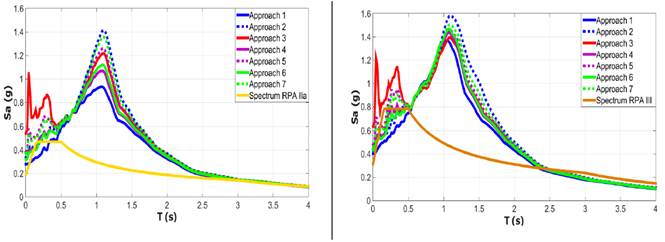
Figure 7 Floor response spectra at the roof level of building calculated from response history analysis for (a) 0.188g, (b) 0.313g
Before the fundamental period of the building which is equal to 0.52 s, we find that the spectral acceleration at the roof level for the mass proportional damping is the most pronounced for the two seismic intensities. As well as the spectral floor acceleration at the roof level for the initial stiffness proportional damping is the least pronounced for the two seismic intensities. In addition, the floor spectral accelerations for tangential Rayleigh damping are the closest to the spectral accelerations of the RPA spectra corresponding to the fundamental period of the building.
4.3 Floor displacements
Figure 8 presents the mean values of maximum floor displacements obtained using different damping approaches and pushover analysis for two seismic intensity measures.
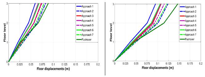
Figure 8 Maximum floor displacements calculated from response history analysis for (a) 0.188g, (b) 0.313g
For the RC building studied, very similar maximum floor displacements are obtained for all damping approaches.
The seismic performance is strongly marked by the first mode with very modest contribution from the higher modes. We obtained globally the same damping matrix for different approaches.
In pushover analysis, the maximum displacements in the second and third levels are superior relative to the nonlinear time history analysis. Particularly in seismic intensity measurements of 0.313 g. In nonlinear time history analysis, seismic ground motion is reduced by the use of a damping matrix.
Different approaches yielded structural responses whose amplitude differences in maximum floor displacements were quantified by calculating ratios for two measurements of seismic intensities. [Table 4].
Maximum floor displacements ratios are calculated as:
% = (Maximum floor displacements - Mean maximum floor displacements) / Mean maximum floor displacements
4.4 Story shear forces
Figure 9 presents the mean values of maximum story shear forces obtained using different damping approaches and pushover analysis for two seismic intensity measures. The same remarks are observed concerning floor displacements.
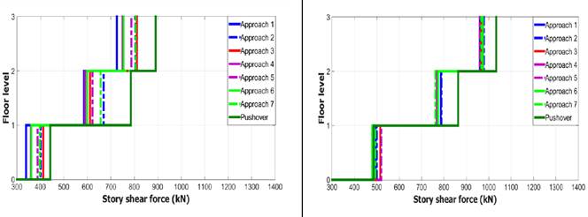
Figure 9 Maximum story shear forces calculated from response history analysis for (a) 0.188g, (b) 0.313g
The differences in magnitude of maximum story shear forces between structural responses obtained with different approaches have been quantified by computing ratios for two seismic intensity measures [Table 5].
Maximum story shear force ratios are calculated as:
% = (Maximum story shear forces - Mean maximum story shear forces) / Mean maximum story shear forces
4.5 Maximum inter-story drift ratio
The inter-story drift performance of a multistory building is an important index of structural and non-structural damage of the building under a range of levels of earthquake motion. The inter-story drift performance has become a principal design consideration in performance design. The system performance levels of a multistory building are evaluated on the basis of the inter-story drift values along the height of the building under different levels of earthquake motion.
The Inter-Story Drift Ratio is evaluated by the Equation (3):
Where
IDR is the inter-story drift
di is the displacement of i story
di-1 is the displacement of i-1 story
hi is the height of i story
Figure 10 presents the mean values of the Inter-story drift ratios obtained using different damping approaches and pushover analysis for two seismic intensity measures.
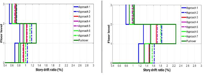
Figure 10 Inter-story drift ratios obtained from response history analysis for (a) 0.188g, (b) 0.313g
The Inter-story drift ratios are more important in the second floors in all approaches; because of the importance of the difference of displacement between the first and the second floor.
Initial and tangent Rayleigh damping models with two approaches result in average Inter-Story Drift Ratio, ratios among mass-proportional and initial and tangent stiffness-proportional damping models.
To reduce Rayleigh damping approach the Inter-Story Drift Ratio is more important compared to Rayleigh damping approach. The reduction of frequencies generates the amplification on the periods, causing attenuation of the damping matrix.
The differences in magnitude of Inter-story drift between structural responses obtained with different approaches have been quantified by computing ratios for two seismic intensity measures [Table 6].
Maximum Inter-story drift ratios are calculated as:
% = (Inter-story drift - Mean inter-story drift) / Mean inter-story drift
5. Conclusions
The investigation of the imports of modeling viscous damping nonlinear time history analysis of RC buildings by different approaches is evaluated using the response of a three-story building.
Lowest damping force/mass force ratios are given by the initial stiffness matrix. Coefficients α and β are constant and independent, with the time. The mass forces and the damping forces were limited because they are proportional to the initial stiffness matrix. Furthermore, mass-proportional damping implies highest damping force/base shear force ratios for different seismic intensity measures for RC frame buildings.The damping force/base shear force ratios resulting from the use of mass-proportional damping model intensificates with a growth in the seismic intensity unlike damping force/base shear force ratios obtained using stiffness-proportional damping which remains constant.
Initial damping reduces the engineering demand parameters. It is caused by the invariability of the damping throughout the analysis.
The Rayleigh damping approach gives smaller maximum engineering demand parameters ratios. [Table 4, Table 5 and Table 6]. It places the different results in the analysis of performance between mass-proportional and stiffness-proportional damping models.
The reduced Rayleigh damping leads to more important results in the analysis of performance compared to Rayleigh damping approach. The reduction of frequencies generates the amplification on the periods, causing attenuation of the damping matrix.
The interpretation of results recapitulated in this article recommends that neither mass-proportional nor stiffness proportional damping are appropriate for inelastic nonlinear time history analysis of RC buildings.
The damping model used in the nonlinear dynamic do not have a significant influence the Inter-Story Drift ratio in the RC buildings according to RPA2003 [40] which represents the low-rise buildings. With the models examined, tangent Rayleigh damping appears to be the ideal alternative option for the RC frame buildings.


