


 English (pdf)
 Article in xml format
 Article references
 Send this article by e-mail
 Cited by SciELO
  Cited by Google
  Similars in
SciELO
Similars in
SciELO  Similars in Google
 Permalink
1. Introduction
The upheaval buckling response of buried submarine pipelines has been a topic of great intereset during the last decades[1-4]. Over the last few years, several projects involving the design, fabrication, and installation of submarine pipelines have been developed in the oil & gas industry. Difficulties arise when the pipe is subjected to high-temperature combined with high-pressure conditions. Catastrophic failures of the pipelines may occur when these conditions are not considered in the design process. Burying a pipeline on the seabed provides good structural stability against hydrodynamic loads; however, it imposes a significant restriction on the longitudinal pipe movement due to thermal expansion. It also leads to an increase in the axial compressive load in the pipe and buckling failure risk if imperfections are present. The main objective in buried pipeline design is to avoid global buckling, since this condition is considered as failure. A buckled pipeline moves vertically out of the seabed, being exposed to the external conditions, and subjected to additional bending stresses at the buckled anchor.
In buried pipelines design, the main objective is to calculate the cover height. Recommendations for offshore pipeline design as recommended by [5] are available, where many guidelines and practical information can be found. The cover design process starts by collecting data from the installation trench to establish the initial configuration, because the out-of-straightness is a key parameter in the buckling response.
A first approach in buried pipeline analysis is to obtain the soil vertical uplift resistance per unit length, which can be achieved by means of experimental, analytical, and numerical works. A model to predict the peak uplift resistance U of buried pipes based on a vertical slip surface mechanism was proposed by [6]. The model parameters are the earth pressure coefficient, K0, to account for normal stresses in slip surfaces, the internal friction coefficient of the soil, ϕ, the effective soil unit weight, γ′, the depth to centerline of the pipe, H, and the pipe diameter, D0. This model is described by Equation (1)

In [7], a model is presented for the peak uplift resistance considering an inclined slip surface mechanism instead of a vertical one, representing a mass block of trapezoidal-shape above the pipe [Figura. 1]. Normal stresses are accounted for by means of lateral earth pressure, the trapezoidal-shape of the block is given by the soil dilatancy, ψ, and the internal friction coefficient controls the shear resistance.
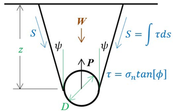

This model is given in Equation (2) and confirms experimental results obtained by the authors Experimentally displacements of buried pipes were obtained in [8]. The soil resistance to pile loading was analyzed in [9] using the Extended Drucker-Prager (EDP) constitutive model, obtaining results in agreement with previous experimental works. Additionally, comparisons between the different approximations were made to obtain EDP model parameters to fit the Mohr-Coulomb failure envelope.
From these models, [1] recommends the calculation of the soil uplift resistance in function of soil characteristics. In practice, this resistance is given as a function of pipe dimensions and cover height. On the other hand, given the soil resistance, the critical axial load can be calculated using an analytical approach provided in [10]. Finally, to conclude the approach proposed by [5], a check is carried out to verify pipe integrity. However, this approach is limited by the fact that only the linear behavior of material is addressed and the complete soil behavior is not considered, hence, a detailed FEM analysis is needed to evaluate this phenomenon.
Focusing on the buckling phenomena, numerous works have been carried with the aim of study the buckling response of a buried pipeline. [11] solved the upheaval buckling problem for pipelines with soft seabed, obtaining differences from rigid seabed solution under certain conditions of rigidity parameter. [12] addressed the differences and limitations of different numerical models to solve the global buckling of pipelines, highlighting the capability of a 3D model to capture the complete response and the pipe-soil interaction. In [13] analytical solutions were compared for the buckling problem with non-linear numerical solutions considering pipe-soil interaction effect obtaining that buckling develops at the zone where the most critical imperfection is found. The critical stress field at the pipe wall due to bending in the buckled zone was also highlighted. [14] developed a dimensional analysis of the buckling problem to study numerically the initial imperfection shape and amplitude effect, obtaining that imperfection shape has an effect in the buckling load besides the amplitude.
[15] focused on the soil behavior working with beam-spring models to fully model the buried pipeline using clay fill, the results showed good agreement with their experimental work with an emphasis in the soil uplift response in terms of the consolidation characteristics. Working with loose sands, [16] showed the dependence between uplift resistance and soil properties. Summing up, these works suggest that the complex soil-pipe interaction can be modeled in a certain way to extract the soil uplift resistance required to study the buckling response of a buried pipeline. However, a complete buckling study of a buried pipeline with the soil interaction effect is needed to obtain the coupled buckling response.
In this work, a nonlinear finite element analysis is carried out considering the complete soil behavior. The model accounts for friction, shear resistance, and downward stiffness for the soil and steel plasticity for the pipeline to obtain the critical buckling load in terms of the initial configuration. Finally, from the numerical results, a mechanical model to determine the buckling load of a buried pipeline is proposed. This model consists of a simply supported beam subject to a distributed lateral load representing the soil uplift resistance, and an axial compressive load modeling the effective axial force following the DNV-RP-F110 recommendations. The mechanical model is developed using the energy method proposed in [17], where the potential energy of the system is expressed as a function of a half sine wave deformed shape. Equilibrium states of the system are obtained searching for the stationary values of potential energy, and then any parameter of interest can be obtained. The strain energy accumulated in the beam is considered using the first order beam theory. In this manner, the initial imperfection can be handled in a more generalized way since it is considered by means of the pipe initial curvature instead of an out-of-straightness amplitude. The initial curvature is easily determined from the laid configuration or pipe route.
2. Numerical modeling
In the design of a submarine pipeline several loading conditions need to be considered such as: internal pressure, external pressure, hydrodynamic loads, and thermal loads. Submarine pipelines are often buried to protect them against hydrodynamic effects, but the high constraint due to the friction with the soil cover makes them more susceptible to thermal effects. In some cases, a pipe needs to be insulated to prevent heat loss and drops in fluid temperature due to process requirements. Additionally, buried pipes might have a concrete cover over partial lengths to increase self-weight and diminish buoyancy. To simplify the numerical models, stiffness effects of the pipeline cover are neglected, and only aggregated weight is used. According to DNV-RP-F110, the compressive axial load is expressed applying the concept of effective axial force S e given by Equation (3).

Where HL is the residual laid tension, At is the cross-sectional area of the pipe, E is the modulus of elasticity, ∆Pi is the internal pressure difference compared to as laid, Ai is the internal cross-sectional area of the pipe, v is the Poisson ratio, α is the thermal expansion coefficient, and ∆T is the temperature difference.
Using this formulation, a single load-displacement analysis can be done considering pressure load explicitly, since it is already accounted for within the effective force concept. The uplift resistance due to soil cover is composed by the block weight and internal friction coefficient. For that reason, modeling the soil cover uplift resistance as a distributed constant load of equal magnitude than the uplift resistance can be used to simplify the problem.
A finite element model is elaborated to determine the buckling load of a buried pipeline. The geometry is generated by sweeping the pipe and soil cross section along a curved path. The pipe dimensions are D o =36 in (0.914m) and t=1 in (0.0254m). The pipe material is an API 5L X65 steel [18], typical specification in offshore industry. This steel has an elastic-plastic behavior that must be considered because the buckling involves large deformations. The data for modeling are based on Ramberg-Osgood stress-strain relationship obtained for this material specification by [19] through experimental tests Equation (4).

Where the yield strength of the pipe is σy=420MPa, the Ramberg-Osgood fitting exponent n=20, Young’s modulus E=207GPa, and Ramberg-Osgood coefficient αR=3/7.
The mechanical behavior and failure criterion of the soil are defined using a simple model based on Coulomb friction law. The failure occurs when a slip plane is generated inside the material, and a relatively rigid body displacement between particles takes place [20]. In this work, in the absence of own field data, the recommended value of parameters given by [1] and common soil properties given by [20] are used. Table 1 shows the corresponding values for clay soils.

From a numerical point of view, the soil is a material with a nonlinear response where the shear strength depends on normal compressive stresses, this means hydrostatic stresses. The yield surface can be expressed by means of Mohr-Coulomb theory and the tensile strength depends of cohesion forces. The plastic behavior of the soil is implemebted through the EDP model available in [21]. Linear functions were selected for yielding F and flow potential Q (Equations (5) and (6)], as the simplest way to define the model


where q is the soil cohesion. The parameters for this model were calculated from Table 1, using a compromise cone approximation to Mohr-Coulomb envelope of the yielding surface as proposed in [9] with (Equations (7) and (8)]. The EDP model coefficients αs and βs are calculated in terms of the internal friction coefficient ϕ and the dilatancy ψ


After substituting the corresponding values for ϕ and ψ given in Table 1, the parameters αs=1.0 and βs=0.94 are attained. The cohesion force q is implemented as the initial yield stress of material σy, and is constant, meaning a perfectly plastic hardening behavior. It gives the soil resistance to tensile loads. The soil density is reduced to account for the buoyancy effect. Thehardening law used in the EDP model cannot represent the strain softening exhibited by soils after reaching the peak force during test experiments. In spite of this, since peak force is characterized by a peak friction coefficient, the critical friction coefficient is used herein, giving a conservative approach to peak responses.
After conducting a convergence analysis, pipe and soil geometries are meshed using Shell 281 and Solid 186 elements, respectively, available in the ANSYS element library [21]. To model the interface between soil and pipe, the interaction is defined as frictional contact with a friction coefficient μ=0.6 according to [1]. The upheaval buckling has a symmetry plane aligned which the vertical axis. Figure 2 shows the boundary conditions considered to solve the problem.
The soil under the pipeline is necessary to support the pipe before buckling occurs for the distributed load model. The curved path is generated which a circumference arch of 100m length, this guarantees a constant curvature along pipe trail. Finally, a convergence analysis is carried out, and the mesh configuration is defined using 6 divisions in the circumference as shown in Figure 2a.
The buckling force was determined from a large deflection analysis by FEM using both the buried pipe model (B. Pipe) and the distributed load model (D. Load) proposed in this work, obtaining that the distributed load model represents appropriately the buckling behavior of the buried pipe model (see Figure 3].
Both models have the same response to the increase of uplift resistance and the initial curvature. The load decreases as initial curvature increases, and the length of buckled pipe arch increases with the increment of the initial curvature. This behavior makes the response of the system be independent of boundary conditions at the pipe ends, since the buckling arch is lesser than model length.
In the classical Euler buckling model the length of the beam is very important. Here the presence of a transversal load acting in the opposite direction of deformation, changes considerably the response, this behavior is studied in the next section. As seen in Figure 3, a good agreement in the results using both numerical models attained, it conveys to the possibility of developing a simple mechanical model capable to represent the buried pipeline buckling phenomena.
3. Mechanical pipe model
The mechanical model for buried pipeline buckling is based on the following assumptions: a) pipe diameter and thickness remains constant, meaning that the pipe beam properties are constant, the pipe material is linear elastic, b) the distributed load over pipe is supposed to be constant, although real soil cover could have depth and composition variations that affect uplift resistance, c) the lateral and downward buckling modes are neglected since the soil restraint in these directions is higher, d) the initial configuration is assumed as a sine wave, being a good approximation to any shape for small curvatures, and e) the beam rests over floor, before axial load is applied, giving support to transverse load.


Figure 3 Comparison between behavior of buried pipeline (B. Load) and pipe under distributed loads (D. Load)
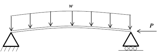
Figure 4 shows a schematic view of the problem to solve. A buried pipeline problem can be simplified and modeled as a simply supported beam under a constant distributed load. The submerged weight of covered pipe and the vertical uplift resistance of soil cover give the magnitude of this distributed load.
Since the buckling phenomenon is an instability problem, the upheaval buckling is solved using this approach in order to handle the initial pipe configuration in a better way. The deformed shape of a buckled buried pipeline is similar to a buckled Euler beam. Hence, the first buckling mode of a pin-ended beam is used to solve the problem, as the fundamental case solution, in order to apply the energy method proposed by [17].
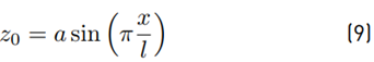
he deflection curve of a pin-ended column is the sine arch given by Equation (9), where z is the deflection, x the position, a the arch height and l the beam length. This curve is supposed to be the initial shape of the model.
After loading, the deflection curve of the beam in the deformed state is given by Equation (10). There, the arch height α is increased by a small quantity b.

The potential energy of the system Π(b) is given by the strain energy of bending and axial deformation, the work done by the external loads, that is, the axial compressive load P, and the distributed load w. This energy is a function of b, the deformed state of the system, and is given by Equation (11).

Additionally, the change in length (∆l) due to the arch rise given in Equation (12) was calculated using a power series approximation (12), and ∆c is the change in curvature given in Equation (13)


Developing the integrals, a final expression for the potential energy II(b) is obtained in Equation (14).

The equilibrium stages of the system are obtained, minimizing the potential energy Π(b) with respect to [∂Π(b)/∂b = 0]. Hence, making the derivative equal to zero, the axial load P (b) of equilibrium is obtained by Equation (15).

The axial strain energy is usually neglected in beam analysis. In this work, the effect of this parameter will be reviewed. However, Equation (16) shows a simplified form of Equation (15), making At = 0. The first term in this equation is the same of the buckling solution of beam with an initial curvature previous obtained by [17]. The second term contains the effect of distributed transverse load, which increases the axial force required to deform the pipeline, and P cr is the classical buckling load.

For practical purposes, the parameter a cannot be easily measured from a pipe run; hence, the curvature (second derivative of the pipe trajectory) is used to measure the initial configuration. The curvature is calculated from the deformed shape given by Equation (9). The following expression Equation (17) is used to determine the amplitude 𝑎 at the beam middle, where the maximum curvature is present. The initial curvature is γ.

Substituting Equation (17) into Equation (16), a new expression for the equilibrium force is obtained as a function of the initial curvature, given by Equation (18).

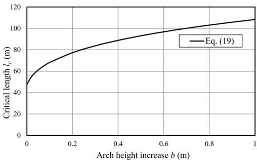
In Equation (16) the distributed load term increases the buckling load with l 2 . Figure 5 shows the results explaining this situation using the data from Table 2. There is a critical length l c where the buckling load is minimal, for a given configuration. This load depends of initial configuration and distributed load magnitude. Hence, in a long pipe system, if this load is achieved the pipe will buckle in a length arch l c .


The length l c given by Equation (19) can be obtained from Equation (18)

The critical force expression Equation (20) is obtained substituting Equations [19,18].

As seen in Figure 6, the arch length increases with 𝑏, it means that the buckled zone length increases, but the equilibrium force decreases with 𝑏 as the typical response in a post-buckling behavior, as seen in Figure 7.
The load-displacement response obtained from the mechanical model shown in Figure 7 has negative slope, meaning that equilibrium state only exists if the system is load-controlled. This stability condition can be checked by Equation (17), obtained through the derivative of Equation (18) with respect to 𝑏. Solving for 𝑤, Equation (21) is found:

The meaning of wo is shown in Figure 8 where the example geometry with l=50m is plotted.


An important change in the system response is obtained for smaller values than w o because the system response is always stable and similar to that from classical buckling theory. However, for values higher than w o , the system response is unstable, because the equilibrium load is higher than classical Euler buckling load. Stability could be achieved if the axial strain energy is not neglected, as can be seen for the curve corresponding to At = 0.05m2 in Figure 8, but the consistency obtained for small deformations makes this assumption valid. The load required for b = 0 is the load needed to separate the beam from the floor (at initial state, the transverse load is all supported by the floor).
The objective of [1] in buried pipe design is to prevent upheaval buckling, meaning that the pipeline must remain under an allowable deformation b resting on the floor. Hence, lateral load must be large enough to prevent vertical displacements for a given effective axial load.
The design of a buried pipeline is aimed at calculating the pipe cover height to prevent the upheaval buckling. For a given problem, the effective axial load can be determined using Equation (3) with P=S. If the pipe route is known the initial curvature at any point can be estimated. The only unknown in the problem is the distributed load 𝑤 given by Equation (22), which can be calculated for design cover height using as example the model proposed by [7] (Equation (2)].

4. Results
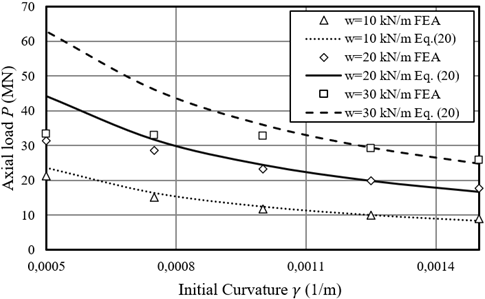
Figure 9 shows the results obtained theoretically using Equation (20) and numerically, varying the initial curvature and distributed load amplitude, of the pipe with Do=36in (0.914m) and t=1in (0.0254m). These results are consistent with the analytical solution in the elastic range, since the finite element model considers steel plasticity and yields to different result for this case. Material plasticity makes pipe to buckle at lower loads due to local yielding. Buckling in the plastic range of material is not desirable and is not investigated in this work.

Another important fact is that the initial configuration of the finite element model is a circumference arch, while the analytical model uses a sine wave, meaning that this assumption leads to good results. The force P is calculated in a deformed state b= 0.02m. A similar result is presented in Figure 10 for the pipe with Do=30in (0.762m), and t=1in (0.0254m). A good agreement for the solution until steel yielding was obtained.

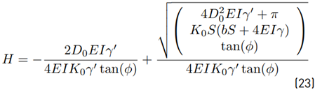
Coupling Equation (21) with Equation (1) leads to obtain Equation (23), then a compact expression is attained for the soil cover height H.
The cover height obtained with Equation (23) is plotted in Figure 11 for a pipe with Do=36in (0.914m) and t=1in (0.0254m), considering different axial loads S, and soil properties: ϕ=30°, γ′ = 1500kg/m3, K0=1. Using this formulation, any soil uplift resistance model can be coupled to obtain cover height to prevent upheaval buckling. Additional experimental work is needed to obtain a better validation of the model. Also, this buckling model can be used to solve global buckling problems for even or uneven seabed. The main difference with buried pipelines is that even on a seabed scenario the transverse load is built from lateral soil friction, and on an uneven seabed scenario, the vertical transverse load is only the submerged weight of the pipeline.
5. Conclusions
Buried pipelines can be modeled as a pipe inside a block mass to consider soil cover effects. This model can be simplified as a simply supported beam under a distributed load, with similar boundary conditions. The numerical results obtained from the full and the simplified model were in good agreement in all aspects. The proposed theoretical model considering a simply supported beam under a lateral distributed load solved the problem, obtaining results consistent whith numerical results.
The usage of the first buckling mode of a pin-ended beam as the fundamental case solution to apply the energy method proposed by Timoshenko provided good results, although the initial shape in the numerical model is different. This led to concluded that for small curvatures the shape approximation is valid.
A critical anchor length where the buckling axial load is minimal for a given configuration was obtained, making the solution suitable for long pipe systems. In classical buckling, the beam length affects the buckling load. The minimal axial load at the critical length was consistent with the results obtained numerically, where the boundary conditions in the numerical model did not affect the solution.
Buckling loads were obtained in terms of pipe properties, initial configuration, and transverse load. Hence, the magnitude of the transverse load can be calculated considering the effective axial load as the buckling load, to prevent pipe uplift. An expression to obtain cover height was obtained coupling buckling solution with soil uplift resistance model. This model provided a design criterion to prevent upheaval buckling. Further validation for the model is needed since the proposed mechanical model was only compared with a numerical solution in the absence of experimental work.

